Borg System Architecture

November 7, 2017November 7, 2017 by rawkintrevo, posted in Engineering, flink, How-Tos, mahout

or “how I accidentally enslaved humanity to the Machine Overlords”.

The Borg are a fictional group from the Sci-Fi classic, Star Trek, who among other things have a collective consciousness. This creates a number of problems for the poor humans (and other species) that attempt to resist the Borg, as they are extremely adaptive. When a single Borg Drone learns something, its knowledge is very quickly propagated through the collective, presumably subject to network connectivity issues, and latency.

Here we create a system for an arbitrary number edge devices to report sensor data, a central processor to use the data to understand the environment the edge devices are participating in, and finally to make decisions / give instructions back to the edge device. This is in essence what the Borg are doing. Yes, there are some interesting biological / cybernetic integrations, however as far as the “hive mind” aspect is concerned, this is basic principles in play.

I originally built this toy to illustrate that “A.I.” has three principle components: Real time data going into a system, an understanding of the environment is reached, a decision is made. (1) Real Time artifical intelligence, like the “actual” intelligence it supposedly mimics is not making E.O.D. batch decisions. (2) In real time the system is aware of what is happening around it- understanding its environment and then using that understanding to (3) make some sort of decision about how to manipulate that environment. Read up on definitions of intelligence, a murky subject itself.

Another sweet bonus, I wanted to show that sophisticated A.I. can be produced with off-the-shelf components and a little creativity, despite what vendors want to tell you. Vendors have their place. It’s one thing to make something cool, another to productionalize it- and maybe you just don’t care enough. However, since you’re reading this- I hope you at least care a little.

Artificial Intelligence is by no means synonymous with Deep Learning, though Deep Learning can be a very useful tool for building A.I. systems. This case does real time image recognition, and you’ll note does not invoke Deep Learning or even the less buzz-worthy “neural nets” at any point. Those can be easily introduced to the solution, but you don’t need them.

Like the Great and Powerful Oz, once you pull back the curtain on A.I. you realize its just some old man who got lost and creatively used resources he had lying around to create a couple of interesting magic tricks.

System Architecture

OpenCV is the Occipital Lobe, this is where faces are identified in the video stream.

Apache Kafka is the nervous system, how messages are passed around the collective. (If we later need to defeat the Borg, this is probably the best place to attack- presuming we of course we aren’t able to make the drones self aware).

Apache Flink is the collective consciousness of our Borg Collective, where thoughts of the Hive Mind are achieved. This is probably intuitive if you are familiar with Apache Flink.

Apache Solr is the store of the “memories” of the collective consciousness.

The Apache Mahout library is the “higher order brain functions” for understanding. It is an ideal choice as it is well integrated with Apache Flink and Apache Spark

Apache Spark with Apache Mahout gives our creation a sense of conext, e.g. how do I recognize faces? It quickly allows us to bootstrap millions of years of evolutionary biological processes.

A Walk Through

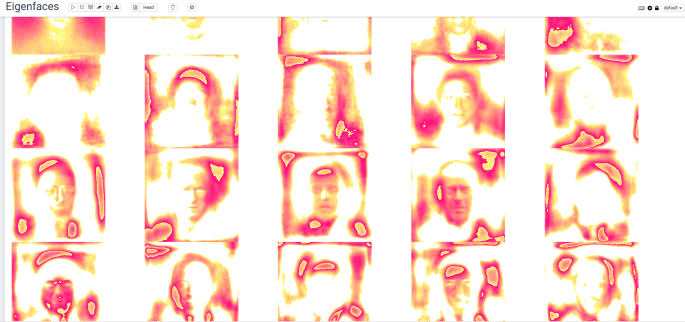
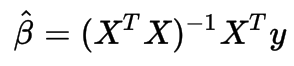
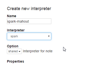
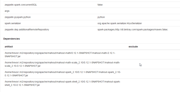
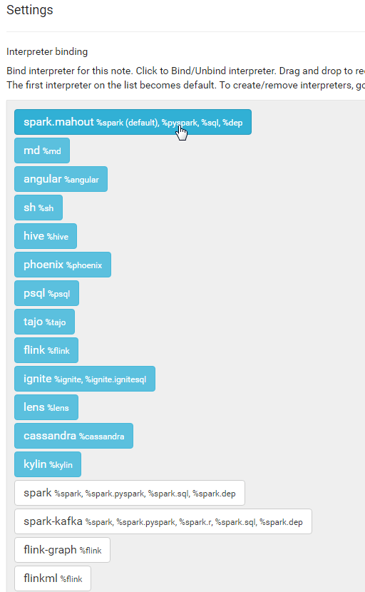
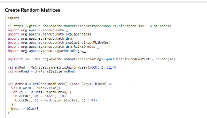
(1) Spark + Mahout used to calculate eigenfaces (see previous blog post).

(2) Flink is started, it loads the calculated eigenfaces from (1)

(3) A video feed is processed with OpenCV .

(4) OpenCV uses Haar Cascade Filters to detect faces.

(5) Detected faces are turned in to Java Buffered Images, greyscaled and size-scaled to the size used for Eigenface calculations and binarized (inefficient). The binary arrays are passed as messages to Kafka.

(6) Flink picks up the images, converts them back to buffered images. The buffered image is then decomposed into linear a linear combination of the Eigenfaces calculated in (1).

(7) Solr is queried for matching linear combinations. Names associated with best N matches are assigned to each face. I.e. face is “identified”… poorly. See next comments.

(8) If the face is of a “new” person, the linear combinations are written to Solr as a new potential match for future queries.

(8) Instructions for edge device written back to Kafka messaging queue as appropriate.

Problems

A major problem we instantly encountered was that sometimes OpenCV will “see” faces that do not exist, as patterns in clothing, shadows, etc. To overcome this we use Flink’s sliding time window and Mahout’s Canopy clustering. Intuitively, faces will not momentarily appear and disappear within a frame, cases where this happens are likely errors on the part of OpenCV. We create a short sliding time window and cluster all faces in the window based on their X, Y coordinates. Canopy clustering is used because it is able to cluster all faces in one pass, reducing the amount of introduced latency. This step happens between step (6) and (7)

In the resulting clusters there are either lots of faces (a true face) or a very few faces (a ghost or shadow, which we do not want). Images belonging to the former are further processed for matches in step (7).

Another challenge is certain frames of a face may look like someone else, even though we have been correctly identifying the face in question in nearby frames. We use our clusters generated in the previous hack, and decide that people do not spontaneously become other people for an instant and then return. We take our queries from step 7 and determine who the person is based on the cluster, not the individual frames.

Finally, as our Solr index of faces grows, our searches in Solr will become less and less effecient. Hierarchical clustering is believed to speed up these results and be akin to how people actually recognize each other. In the naive form, for each Solr Query will scan the entire index of faces looking for a match. However we can clusters the eigenface combinations such that each query will first only scan the cluster centriods, and then only consider eigenfaces in that cluster. This can potentially speed up results greatly.

Usecases

Borg

This is how the Borg were able to recognize Locutus of Borg.

Cylons

This type of system also was imperative for Cylon Raiders and Centurions to recognize (and subsequently not inadvertently kill) the Final Five.

Shorter Term

This toy was originally designed to work with the Petrone Battle Drones however as we see the rise of Sophia and Atlas, this technology could be employed to help multiple subjects with similar tasks learn and adapt more quickly. Additionally there are numerous applications in security (think network of CCTV cameras, remote locks, alarms, fire control, etc.)

Do you want Cylons? Because that’s how you get Cylons.

Alas, there is no great and powerful Oz. Or- there is, and …

References

Flink Forward, Berlin 2017
Slides Video (warning I was sick this day. Not my best work).

Lucene Revolution, Las Vegas 2017
Slides Video

My Git Repo

PR Donating this to Apache Mahout
If you’re interested in contributing, please start here.

Introducing Pre-canned Algorithms in Apache Mahout

May 2, 2017May 3, 2017 by rawkintrevo, posted in big data for noobs, Engineering, mahout

Apache Mahout v0.13.0 is out and there are a lot of exciting new features and integration including GPU acceleration, Spark 2.x/Scala 2.10 integration (experimental- full blown in 0.13.1), and a new framework for “precanned algorithms”. In this post we’re going to talk about the new algorithm framework, and how you can contribute to your favorite machine learning on Big Data library.

If you’re not familiar with the Apache Mahout project, it might be helpful to watch this video but in short- it allows you to quickly and easily write your own algorithms in a distributed back-end independent (think Apache Spark, Apache Flink, etc), and mathematically expressive extension of the Scala language. Now v0.13.0 allows the user to accelerate their distribute cluster with GPUs (this is independent of Spark- ANY cluster can be accelerated), and lays out a framework of pre-canned algorithms.

Key Concepts

The Algorithms Framework in Apache Mahout, borrows from the traditions of many of the great machine learning and statistical frameworks available today, but most notably- R and Python’s sklearn. When reasonable, Mahout makes a good faith effort to draw on the best parts of each of these.

sklearn – has a very consistent API.
R – is very flexible.
Both are extendable, and encourage users to create and submit their own implementations to be available for other users (via CRAN and Pypi respectively).

Fitters versus Models

The first concept we want to address is the idea of a fitter and a model. Now that I have setup the Mahout Algorithms framework, I instantly point out a major break from the way things are done in R and sklearn. As the great thinkers Ralph Waldo Emerson and the person who wrote PEP-8 said, “A foolish consistency is the hobgoblin of little minds.”

In sklearn, the model and the fitter are contained in the same class. In R, there is an implicitly similar paradigm… sometimes.

Model is an object which contains the parameter estimates. The R function lm generates models. In this way, a Fitter in Apache Mahout generates a model of the same name (by convention. E.g. OrdinaryLeastSquares generates an OrdinaryLeastSquaresModel which contains the parameter estimates and a .predict(drmX) method for predicting new values based on the model.

Recap: A Fitter Generates a Model. A model is an object that contains the parameter estimates, fit statistics, summary, and a predict() method.

Now if you’re thinking, “but why?”, good on you for questioning things. Why this break from sklearn? Why not let the fitter and the model live in the same object? The answer is because at the end of the day- we are dealing in big data, and we want our models to be serialized as small as is reasonable. If we were to include everything in the same object (the fitter, with the parameter estimates, etc.) then when we saved the model or shipped it over the network we would have to serialize all of the code required to fit the model and ship that with it. This would be somewhat wasteful.

Class Heirarchy

The following will make the most sense if you understand class hierarchy and class inheritance. If you don’t know/remember these things, now would be a good time to review.

This isn’t a complete diagram but it is illustrative. For example- all Models have a summary string. All SupervisedModels have a Map of testResults. All RegressorModels have a .predict(...) method, and when ClassifierModel is introduced, they may have a .predict(...) method as well, or perhaps they will have a .classify(...) method.

Preprocessors are treated as unsupervised models. They must also be fit. Consider a StandardScaler, which must be “fit” on a data set to learn the mean and standard deviation.

The hierarchy of fitters is identical.

Hyper-parameter system

Hyper-parameters are passed in fitter functions as symbols. For example:

val model = new OrdinaryLeastSquares[Int]().fit(drmX, drmY, 'calcCommonStatistics → false)

Different methods have different hyper-parameters which maybe set. This method has advantages of extreme flexibility. It also side-steps the type safety of the Scala language, which depending on weather or not you like or hate type-safety, you might consider to be a good or bad thing. A notable draw back- if you pass a parameter that isn’t used by the method, it will be ignored silently, that is to say it will be ignored and it won’t warn you are throw an error. The real threat here is typos- where you think are doing something like, specifying an interceptless regression, however instead of specifying 'addIntercept -> false you accidentally type 'addInterept -> false, then the regression will add an intercept and throw no warnings that you’ve committed a typo. (This will possibly be fixed soon).

Also, in both hyperparameter examples given have had Boolean values, however the value can be anything. For example, in Cochrane-Orcutt on of the hyperparameters 'regressor can be any sub-class of LinearRegressorFitter!

In Practice

Preprocessors

There are currently three pre-processors available.
* AsFactor which is sometimes referred to as Dummy Variables or One-Hot encoder (Mahout chose R-semantics here over Python)
* StandardScaler which is goes by the same name in sklearn and the function scale in R.
* MeanCenter which is very similar to the standard scaler, however it only centers each column. In the future it is possible that MeanCenter will be combined with StandardScaler (as is done in R).

A preprocessor example

A fun tip: the unit tests of any package are full of great example. This one comes from: https://github.com/apache/mahout/blob/master/math-scala/src/test/scala/org/apache/mahout/math/algorithms/PreprocessorSuiteBase.scala

Setup Code

val A = drmParallelize(dense(
(3, 2, 1, 2),
(0, 0, 0, 0),
(1, 1, 1, 1)), numPartitions = 2)

// 0 -> 2, 3 -> 5, 6 -> 9

How to use `AsFactor` from Apache Mahout

val factorizer: AsFactorModel = new AsFactor().fit(A)
val factoredA = factorizer.transform(A)
val myAnswer = factoredA.collect

Check our results

println(factoredA)
println(factorizer.factorMap)
val correctAnswer = sparse(
svec((3 → 1.0) :: (6 → 1.0) :: (8 → 1.0) :: (11 → 1.0) :: Nil, cardinality = 12),
svec((0 → 1.0) :: (4 → 1.0) :: (7 → 1.0) :: ( 9 → 1.0) :: Nil, cardinality = 12),
svec((1 → 1.0) :: (5 → 1.0) :: (8 → 1.0) :: (10 → 1.0) :: Nil, cardinality = 12)
)
val epsilon = 1E-6
(myAnswer.norm - correctAnswer.norm) should be <= epsilon
(myAnswer.norm - correctAnswer.norm) should be <= epsilon

The big call out from the above- is that the interface for this preprocessor (the second block of code) is exceptionally clean for a distributed, GPU accelerated, machine learning package.

Regressors

There are currently two regressors available:
* OrdinaryLeastSquares – Closed form linear regression
* Cochrane-Orcutt – A method for dealing with Serial Correlation

Oh, horay- another linear regressor for big data. First off- don’t be sassy. Second, OLS in Apache Mahout is closed form- that is to say, it doesn’t rely on Stochastic Gradient Descent to approximate the parameter space β.

Among other things, this means we are able to know the standard errors of our estimates and make a number of statistical inferences, such as the significance of various parameters.

For the initial release of the algorithms framework, OrdinaryLeastSquares was chosen because of its widespread familiarity. CochraneOrcutt was chosen for its relative obscurity (in the Big Data Space). The Cochrane Orcutt procedure is used frequently in econometrics to correct for auto correlation in the error terms. When auto-correlation (sometimes called serial-correlation) is present the standard errors are biased, and so is our statistical inference. The Cochrane Orcutt procedure attempts to correct for this.

It should be noted, implementations of Cochrane-Orcutt in many statistics packages such as R’s orcutt iterate this procedure to convergence. This is ill-advised on small data and big data alike. Kunter et. al recommend no more than three iterations of the Cochrane Orcutt procedure- if suitable parameters are not achieved, the user is advised to use another method to estimate ρ.

The point of implementing the CochraneOrcutt procedure was to show, that the framework is easily extendable to esoteric statistical/machine-learning methods, and users are encouraged to extend and contribute. Observe the implementation of the algorithm, and after groking, the reader will see that the code is quite expressive and tractable, and the majority of the fit method is dedicated to copying variables of interest into the resulting Model object.

A Regression Example

Setup Code

val alsmBlaisdellCo = drmParallelize( dense(
(20.96,  127.3),
(21.40,  130.0),
(21.96,  132.7),
(21.52,  129.4),
(22.39,  135.0),
(22.76,  137.1),
(23.48,  141.2),
(23.66,  142.8),
(24.10,  145.5),
(24.01,  145.3),
(24.54,  148.3),
(24.30,  146.4),
(25.00,  150.2),
(25.64,  153.1),
(26.36,  157.3),
(26.98,  160.7),
(27.52,  164.2),
(27.78,  165.6),
(28.24,  168.7),
(28.78,  171.7) ))

val drmY = alsmBlaisdellCo(::, 0 until 1)
val drmX = alsmBlaisdellCo(::, 1 until 2)

Cochrane-Orcutt

var coModel = new CochraneOrcutt[Int]().fit(drmX, drmY , ('iterations -> 2))
println(coModel.beta)
println(coModel.se)
println(coModel.rho)

Regression Tests

Unlike R and sklearn, all regression statistics should be considered optional, and very few are enabled by default. The rationale for this is that when working on big data, calculating common statistics could be costly enough that, unless the user explicitly wants this information, the calculation should be avoided.

The currently available regression tests are
* CoefficientOfDetermination – calculated by default, also known as the R-Square
* MeanSquareError – calculated by default, aka MSE
* DurbinWatson – not calculated by default, a test for the presence of serial correlation.

When a test is run, the convention is the following:

var model = ...
model = new MyTest(model)
model.testResults.get(myTest)

The model is then updated with the test result appended to the model’s summary string, and the value of the test result added to the model’s testResults Map.

Extending

Apache Mahout’s algorithm framework was designed to be extended. Even with the few example given, it should be evident that it is much more extensible than SparkML/MLLib and even sklearn (as all of the native optimization is abstracted away).

While the user may create their own algorithms with great ease- all are strongly encouraged to contribute back to the project. When creating a “contribution grade” implemenation of an algorithm a few considerations must be taken.

The algorithm must be expressed purely in Samasara (The Mahout R-Like DSL). That is to say, the algorithm may not utilize any calls specific to an underlying engine such as Apache Spark.
The algorithm must fit into the existing framework or extend the framework as necessary to ‘fit’. For example, we’d love to see a classification algorithm, but one would have to write the Classifier trait (similar to the Regressor trait).
New algorithms must demonstrate a prototype in either R, sklearn, or someother package. That isn’t to say the algorithm must exist (though currently, all algorithms have an analgous R implementation). If there is no function that performs your algorithm, you must create a simple version in another language and include it in the comments of your unit test. This ensures that others can easily see and understand what it is that the algorithm is supposed to do.

Examples of number three are abound in the current unit tests. Example

Conclusions

Apache Mahout v0.13.0 offers a number of exciting new features, but the algorithms framework is (biasedly) one of my favorite. It is an entire framework that encourages statisticians and data scientists who have until now been intimidated by contributing to open source a green field opportunity to implement their favorite algorithms and commit them to a top-level Apache Software Foundation project.

There has been to date a mutually exclusive choice between ‘powerful, robust, and extendable modeling’ and ‘big data modeling’, each having advantages and disadvantages. It is my sincere hope and believe that the Apache Mahout project will represent the end of that mutual exclusivity.

Lucky Number 0.13.0

April 18, 2017 by rawkintrevo, posted in mahout

Apache Mahout has just released the long awaited 0.13.0 which introduces modular native solvers (e.g. GPU support!).

TensorFlow has done a great job driving the conversation around bringing GPU accelerated linear algebra to the masses for implementing custom algorithms, however it has a major draw back that it prefers to manage its own cluster or can work on top of Apache Spark. Mahout on the other hand was designed to work on top of Spark or with any user defined distributed back-end (it just so happens Spark is the generic one we recommend for people trying out Mahout- but if you happen to use Spark great, you’re all set!)

Mahout for Hybrid Spark-GPU clusters

In Mahout, we strive to make everything modular, use something off the shelf or write your own that is optimized to you environment. In 0.13.0 Mahout has introduced a concept of modular native solvers. The native solver is a what gets called when you do any BLAS Like operations (e.g. matrix-matrix multiplication, matrix-vector multiplication, etc.). Many machine learning packages such as R, Python’s sklearn, and Spark’s MLLib utilize Fortran based solvers for speeding up these types of operations. The two native solvers currently included in Mahout are based on ViennaCL, which allow the user to utilize GPUs (via the org.apache.mahout:mahout-native-viennacl_2.10:0.13.0 artifact) or CPUs (via the org.apache.mahout:mahout-native-viennacl-omp_2.10:0.13.0 artifact).

A quick review on how Mahout works under the hood

To understand how this gets used in practice, let’s review how Mahout does math on a Distributed Row Matrix (DRM). A DRM is really a wrapper for an underlying data structure, for example in Spark a RDD[org.apache.mahout.math.Vector]. When we do some math in Mahout on a DRM, for example

drmA %*% incoreV

We are taking a DRM (which is wrapping an RDD) and taking the dot product of each row. In Spark for instance, each executor is multiplying every row of each partition it has locally by a vector (taking the dot product), this happens in the JVM.

When a native solver such as ViennaCL is in use, each executor attempts to use the ViennaCL library to dump the data out of the JVM (where the exectutor is running), utilize a GPU if one exists, load the data into the GPU and execute the operation there. (GPUs are super charged for BLAS operations like this).

This works in a similar way using ViennaCL-OMP, the difference is that all available CPUs are used.

On a Spark-GPU hybrid cluster

Supposing then you have a Spark cluster, and on each node there are GPUs available- then what you now have is statistics/machine learning on Spark which is GPU accelerated. If you have some other distributed engine that executed in the JVM (such as Apache Flink) then you also get GPU acceleration there!

If you don’t have GPUs on your Spark Cluster, you can also use the ViennaCL-OMP package to see significant performance gains. It should be noted though, the optimal ‘tuning’ of one’s Spark jobs changes when using OMP. Since ViennaCL-OMP will utilize all available CPUs, it is advised to set the partitioning of the DRM to be equal to the number of nodes you have. This is because they way Spark normally paralellizes jobs is by using one core per partition to do work- however, since OMP will invoke all cores, you don’t gain anything by ‘over parallelizing’ your job. (This assumes that setting partitions = number of executors will still allow your full data set to fit in memory).

Other cool stuff

In addition to the super-awesome GPU stuff, there are also a couple of other fun little additions.

Algorithms Framework

Currently this is very sparse, but represents Mahout moving toward offering a large collection of contributed algorithms via a consistent API similar to Python’s sklearn.

Consider classic OLS.

val drmData = drmParallelize(dense(
  (2, 2, 10.5, 10, 29.509541),  // Apple Cinnamon Cheerios
  (1, 2, 12,   12, 18.042851),  // Cap'n'Crunch
  (1, 1, 12,   13, 22.736446),  // Cocoa Puffs
  (2, 1, 11,   13, 32.207582),  // Froot Loops
  (1, 2, 12,   11, 21.871292),  // Honey Graham Ohs
  (2, 1, 16,   8,  36.187559),  // Wheaties Honey Gold
  (6, 2, 17,   1,  50.764999),  // Cheerios
  (3, 2, 13,   7,  40.400208),  // Clusters
  (3, 3, 13,   4,  45.811716)), numPartitions = 2)


val drmX = drmData(::, 0 until 4)
val drmY = drmData(::, 4 until 5)

import org.apache.mahout.math.algorithms.regression.OrdinaryLeastSquares

var model = new OrdinaryLeastSquares[Int]()
model.fit(drmX, drmY)
model.summary

Which returns:

res3: String = 
Coef.       Estimate        Std. Error      t-score         Pr(Beta=0)
X0  -1.336265388326865  2.6878127323908942  -0.49715717625097144    1.354836239139669
X1  -13.157701320678825 5.393984138816236   -2.4393288860442244 1.9287400286811958
X2  -4.152654199019935  1.7849055635870432  -2.326540005105108  1.9194430753543341
X3  -5.67990809423236   1.886871957793384   -3.0102244462177334 1.960458377021527
(Intercept) 163.17932687840948  51.91529676169986   3.143183937239744   0.03474107366050938

Feels just like R, with the one caveat that X0 is not the intercept- a slight cosmetic issue for the time being.

The following algorithms are included as of 0.13.0:

Preprocessing
– AsFactor: Given a column of integers, returns a sparse matrix (also sometimes called “OneHot” encoding).
– MeanCenter: Centers a column on its mean
– StandardScaler: Scales a column to mean= 0 and unit variance.
Regression
– OrdinaryLeastSquares: Closed form ordinary least squares regression
Remedial Measures
– CochraneOrcutt: When serial correlation in the error terms is present the test statistics are biased- this procedure attempts to ‘fix’ the estimates
Tests
– Coefficent of Determination: Also known as R-Squared
– MeanSquareError
– DurbinWatson: Tests for presence of serial correlation

MahoutCollections

This is a small package that adds Scala-like methods to org.apache.mahout.math.Vector. Specifically it adds the toArray and toMap method.

While these may seem trivial, I for one have found them extremely convenient (which is why I contributed them 🙂 )

Spark DataFrame / MLLib convenience wrappers.

Spark can be a really useful tool for getting your data ready for Mahout- however there was a notable lack of methods for easily working with DataFrames or RDDs of org.apache.spark.mllib.linalg.Vector (the kinds of RDD that MLLib likes).

For convenience, the following were added:
–drmWrapMLLibLabledPoint
–drmWrapDataFrame
–drmWrapMLLibVector

drmWrapMLLibLabledPoint

val myRDD: RDD[org.apache.spark.mllib.regression.LabeledPoint] = ...
val myDRM = drmWrapMLLibLabeledPoint(myRDD)
// myDRM is a DRM where the 'label' is the last column

drmWrapDataFrame

val myRDD: RDD[org.apache.spark.mllib.linalg.Vector] = ...
val myDRM = drmWrapMLLibVector(myRDD)

drmWrapMLLibVector

val myDF = ... // a dataframe where all of the values are Doubles
val myDRM = drmWrapDataFrame(myDF)

Conclusions

This was a really hard fought release, and an extra special thanks to Andrew Palumbo and Andrew Musselman. If you see them at a bar, buy them a beer; if you see them at a taco stand, buy them some extra guac.

Apache Mahout! What’s Next? DFW Big Data Meetup Talk

December 19, 2016 by rawkintrevo, posted in mahout, video

Deep Magic, Volume 3: Eigenfaces

November 10, 2016November 11, 2016 by rawkintrevo, posted in big data for noobs, Engineering, How-Tos, mahout

This week we’re going to really show off how easy it is to “roll our own” algorithms in Apache Mahout by looking at Eigenfaces. This algorithm is really easy and fun in Mahout because Mahout comes with a first class distributed stochastic singular value decomposition Mahout SSVD.

This is going to be a big job, and assumes you are have HDFS, and a small cluster to work with. You may be able to run this on your laptop, but I would recommend following the last post on setting up a small cloud-based hadoop cluster with Apache Zeppelin.

Eigenfaces are an image equivelent(ish) to eigenvectors if you recall your high school linear algebra classes. If you don’t recall: read wikipedia otherwise, it is a set of ‘faces’ that by a linear combination can be used to represent other faces.

Step 1. Get Data

The first thing we’re going to do is collect a set of 13,232 face images (250×250 pixels) from the Labeled Faces in the Wild data set.

Because some of these shell commands take a little while to run, it is worth taking a moment to set shell.command.timeout.millisecs in the sh interpreter to 600000.

My first paragraph, I’m going to make a directory for my final eigenface images that Zeppelin’s HTML loader can use. Then I’m going to download and untar the dataset. Finally, I’ll put the dataset into the tmp folder in HDFS.

%sh

mkdir zeppelin-0.7.0-SNAPSHOT/webapps/webapp/eigenfaces

wget http://vis-www.cs.umass.edu/lfw/lfw-deepfunneled.tgz
tar -xzf lfw-deepfunneled.tgz
hdfs dfs -put /home/guest/lfw-deepfunneled /tmp/lfw-deepfunneled

Step 2. Add dependency JARs

We use the Scala package scrimage to do our image processing, so we’ll want to add those jars. Also, there is a bug we’re working on in Mahout where broadcasting vectors doesn’t work so well in shell / Zeppelin mode. To get around this, I have added the transformer I need in custom jar of algorithms I use.

MAHOUT-1892: Broadcasting Vectors in Mahout-Shell

If that issue is still open, you’ll need to clone and build my branch (or make your own jar).

git clone https://github.com/rawkintrevo/mahout
cd mahout
git checkout mahout-1856
mvn clean package -DskipTests

Finally, assuming you are using Big Insights on Hadoop Cloud, you’ll need to copy the jar to the cluster.

scp algos/target/mahout-algos_2.10-0.12.3-SNAPSHOT.jar username@bi-hadoop-prod-XXX.bi.services.us-south.bluemix.net:/home/guest/mahout-algos_2.10-0.12.3-SNAPSHOT.jar

Changing username to your username and bi-hadoop-prod-XXX.bi.services.us-south.bluemix.net to your server address.

Back in Zeppelin, load the dependencies:

%sparkMahout.dep

z.load("com.sksamuel.scrimage:scrimage-core_2.10:2.1.0")
z.load("com.sksamuel.scrimage:scrimage-io-extra_2.10:2.1.0")
z.load("com.sksamuel.scrimage:scrimage-filters_2.10:2.1.0")

// add EXPERIMENTAL mahout algos
// https://github.com/rawkintrevo/mahout/tree/mahout-1856/algos
z.load("/home/guest/mahout-algos_2.10-0.12.3-SNAPSHOT.jar")

Step 3. Setup the Mahout Context

This step imports the Mahout packages and sets up the Mahout Distributed Context

%sparkMahout.spark

import org.apache.mahout.math._
import org.apache.mahout.math.scalabindings._
import org.apache.mahout.math.drm._
import org.apache.mahout.math.scalabindings.RLikeOps._
import org.apache.mahout.math.drm.RLikeDrmOps._
import org.apache.mahout.sparkbindings._

@transient implicit val sdc: org.apache.mahout.sparkbindings.SparkDistributedContext = sc2sdc(sc)

Step 4. Create a DRM of Vectorized Images

When doing image processing, we want a Matrix where each image is represented as a vector of numbers, where the number correspond to each pixel.

%sparkMahout.spark

import com.sksamuel.scrimage._
import com.sksamuel.scrimage.filter.GrayscaleFilter

val imagesRDD:DrmRdd[Int] = sc.binaryFiles("/tmp/lfw-deepfunneled/*/*", 500)
       .map(o => new DenseVector( Image.apply(o._2.toArray)
       .filter(GrayscaleFilter)
       .pixels
       .map(p => p.toInt.toDouble / 10000000)) )
   .zipWithIndex
   .map(o => (o._2.toInt, o._1))

val imagesDRM = drmWrap(rdd= imagesRDD).par(min = 500).checkpoint()

println(s"Dataset: ${imagesDRM.nrow} images, ${imagesDRM.ncol} pixels per image")

sc.binaryFiles is the spark way to read in our images. We set out partitioning to 500, and map each image into a scrimage object which drops the color information (we don’t need it for feature mapping) and converts the image to an array of large integers. We scale the integers down, and use the array to create a Mahout DenseVector. Finally we zipWithIndex and then use drmWrap to transform our RDD into a DRM.

Step 5. Subtract Means

IF vector broadcasting in the shell were working (it may be by the time you read this), this is how we would subtract our means.

%sparkMahout.spark

// How you would do this without help
// Doesn't work re BUG: MAHOUT-1892
val colMeansV = imagesDRM.colMeans
val bcastV = drmBroadcast(colMeansV)

val smImages = input.mapBlock(imagesDRM.ncol) {
case (keys, block) =>
      val copy: Matrix = block.cloned
      copy.foreach(row => row -= bcastV.value)
      (keys, copy)
}

We use the .colMeans method to get the colmeans, and then do a mapBlock on the images matrix, subtracting the mean from each image.

Since at the moment the above does not work, here is the hack to do it.

%sparkMahout.spark

// EXPERIMENTAL https://github.com/apache/mahout/pull/246
import org.apache.mahout.algos.transformer.SubtractMean

// Subtract Mean transforms each row by subtracting the column mean
val smTransformer = new SubtractMean()

smTransformer.fit(imagesDRM) // calculuates the column mean
val smImages = smTransformer.transform(imagesDRM) // return new DRM of subtracted means

smImages.checkpoint()

Again, this is only needed as a work around. If you’re interested in how easy it is to package your own functions into a jar- check out the SubtractMean source code

Step 6. Distributed Stochastic Singlar Value Decomposition

Based primarily on Nathan Halko’s dissertation most of the hard part here is done for us.

%sparkMahout.spark

import org.apache.mahout.math._
import decompositions._
import drm._

val(drmU, drmV, s) = dssvd(smImages, k= 20, p= 15, q = 0)

Here k is rank of the output e.g. the number of eigenfaces we want out. p is oversampling parameter, and q is the number of additional power iterations. Read Nathan’s paper or see ssvd docs for more information.

The above will take some time- about 35 minutes on a 5-node Big Insights Cloud Cluster.

drmV will be contain our Eigenfaces (transposed).

drmU will tell us the composition of each face we fed into the algorithm. For example

%sparkMahout

drmU.collect(0 until 1, ::)

yields

{0:-5.728272924185402E-4,1:0.005311020699576641,2:-0.009218182156949998,3:0.008125182744744356,4:0.001847134204087927,5:-0.01391318137456792,6:0.0038760898878500913,7:0.0022845256274037842,8:0.007046521884887152,9:0.004835772814429175,10:0.00338488781174816,11:0.009318311263249005,12:-0.005181665861179919,13:-0.004665157429436422,14:0.003072181956470255,15:-0.01285733757511248,16:0.005066140593688097,17:-0.016895601017982726,18:-0.012156252679821318,19:-0.008044144986630029 ... }

Which implies the first image = .005 * eigenFace1 + -.009 * eigenFace2 + …

Step 7. Write the Eigenfaces to disk

We want to SEE our eigenfaces! We use scrimage again to help us reconstruct our calculated eigenfaces back in to images.

%sparkMahout.spark

import java.io.File
import javax.imageio.ImageIO

val sampleImagePath = "/home/guest/lfw-deepfunneled/Aaron_Eckhart/Aaron_Eckhart_0001.jpg"
val sampleImage = ImageIO.read(new File(sampleImagePath))  
val w = sampleImage.getWidth
val h = sampleImage.getHeight

val eigenFaces = drmV.t.collect(::,::)
val colMeans = smImages.colMeans

for (i <- 0 until 20){
    val v = (eigenFaces(i, ::) + colMeans) * 10000000
    val output = new Array[com.sksamuel.scrimage.Pixel](v.size)
    for (i <- 0 until v.size) {
        output(i) = Pixel(v.get(i).toInt)
    }
    val image = Image(w, h, output)
    image.output(new File(s"/home/guest/zeppelin-0.7.0-SNAPSHOT/webapps/webapp/eigenfaces/${i}.png"))
}

First we load a sampleImage so we can get the height and width. I could have just opened it up in an Image viewer, but y’know, code. drmV has our eigenfaces as columns, so we transpose that. Also recall we subtracted the column means when we in-processed the images, so we’ll need to add that back.

We do a simple for loop over the eigenFaces, basically undoing the inprocessing we did. We then create an array of pixels, we do that by iterating through the vector. Finally we create the image with the width and height, and save it to the directory we set up. ZEPPELIN_HOME/webapps/webapp/ is the root directory for the %html interpreter, so we save our images in a directory there (we created this directory at the beginning).

Step 8. Display the Images

Scala is fun, but for simple string and list manipulation, I love Python

%python

r = 4
c = 5
print '%html\n<table style="width:100%">' + "".join(["<tr>" + "".join([ '<td><img src="eigenfaces/%i.png"></td>' % (i + j) for j in range(0, c) ]) + "</tr>" for i in range(0, r * c, r +1 ) ]) + '</table>'

All that does is create an html table of our images.

And that’s it!

I hope you enjoyed this one as much as I did, please leave comments and let me know how it went for you.

Deep Magic Volume2: Absurdly Large OLS with Apache Mahout

October 13, 2016March 20, 2017 by rawkintrevo, posted in Engineering, How-Tos, mahout, zeppelin

In this post we’re going to really show off the coolest (imho) use-case of Apache Mahout – roll your own distributed algorithms.

All of these posts are meant for you to follow-along at home, and it is entirely possible, you don’t have access to a large YARN cluster. That’s OK. Short story- they’re free on IBM’s BlueMix, where you can:
1. Sign up for a free 30-day account
2. Setup a 5-Node BigInsights (IBMs Hadoop Distro) on Cloud
3. Install Apache Zeppelin and Apache Mahout
4. Run an absurdly large OLS algorithm

The benefit of using a Hadoop as a Service environment is that for analytics, our dataset might not be HUGE enough that uploading is prohibitive, but big enough that we need more horse power than a single node can provide. Being able to spool up a cluster, upload a few files, do some work on it with 5 nodes/240GB RAM/ 48 Virtual processors- and then throw the environment away has a lot of use cases.

In this post we’re doing to write an Ordinary Least Squares algorithm, and then run it on a dataset of 100 million observations by 100 columns (dense).

This is a simplest of algorithms to get you started. Once you have this power at your finger tips, implement any algorithm you find specified in matrix form (which is most of them in academic papers) in Spark or Flink with ease. No longer are you tied to what ever the powers that be running SparkML and FlinkML decide to implement!

Disclosure: I’m working for IBM now, this isn’t an unsolicited sales pitch. The notebook available for part 4 will be available and will run on any Zeppelin instance (assuming you’ve followed the directions for setting up Mahout on Apache Spark listed in a previous post). If you are running Zeppelin locally, you also won’t be able to go as big as we do.

Step 1. Sign up for BlueMix-

Link to Signup

Step 2. Setup a 5-Node BigInsights on Cloud

In short IBM Big Insights on Cloud is Hadoop-as-a-Service. It’s also fairly simple to setup.

There are a few different UIs floating around at the moment, if you can’t find a way to create BigInsights, this link might help (must be logged in). Link

Click on BigInsights. In the next window, there should be a button that says ‘Create’ somewhere towards the right or bottom-right. (Old vs. new UI). From this point on, everything should look the same, so I’ll post more screen shots.

On the next screen click “Open”, and on the screen following that click “New Cluster”.

You should now be at a screen that looks like this:

The cluster name/ username / password don’t really matter.

In the following section, make sure to set the following:

Number of Data Nodes: 5 (current max for free users)
IBM Open Platform Version: IOP 4.2 (4.3 has Spark 2.0- gross).
Optional Components: Make sure Spark is checked.

Click “Create” and then go grab some coffee or whatever. It will take about 5-10 minutes to setup.

After you click create you’ll be taken to a screen talking about your cluster.

In the top center you will see SSH Host and a value below that looks something like bi-hadoop-prod-XXXX.bi.services.us-south.bluemix.net, where the XXXX will be four numbers. You will need this value for the next step.

Step 3. Install Apache Zeppelin and Apache Mahout

As a proud new IBM employee, I get unfettered access to these little clusters, to celebrate I’ve done a little Python witchcraft for quickly installing and my favorite services into BigInsights Cloud instances. These scripts also open up some ports in the firewall as needed for WebUIs (especially on Zeppelin, Apache NiFi, and Apache Flink).

The scripts in essence do the following:
– ssh in to the cluster
– download the binaries of the desired program (Zeppelin, NiFi, Flink, etc.)
– untar the program
– Upload some config files specific to BigInsights
– Start the service
– If a WebUI is necessary, a BlueMix app will be created which establishes an ssh tunnel between the world wide web and the port of the service (e.g. 8080 for Zeppelin).

Skip to the end of this section to see what I mean regarding the BlueMix app.

rawkintrevo’s scripts for installing extra services on BigInsights Cloud on github

The following assumes you are running on some sort of Ubuntu. The principals are the same, but you might need to take different steps to make this work on CentOS or OSX.

Obviously you need Python.

You also need the Python modules paramiko and scp, which are used for using ssh with Python. To install these in Ubunbu, from the command line run:
– sudo apt-get install python-paramiko
– sudo apt-get install python-scp

Next you will need to install Cloud Foundry and IBM’s Cloud Foundry bonus packs.

Install CloudFoundry

IBM BlueMix Docs

On Ubuntu, it’s going to look something like this-

Download Cloud Foundry Installer All Installers:

wget https://cli.run.pivotal.io/stable?release=debian64&amp;version=6.22.1&amp;source=github-rel

Unpack and install Cloud Foundry:

sudo dpkg -i ./cf-cli-*.deb &amp;&amp; apt-get install -f

Set BlueMix Plugin Registry Endpoint:

cf add-plugin-repo bluemix-cf-staging https://plugins.ng.bluemix.net

Install BlueMix Plugins:

cf install-plugin active-deploy -r bluemix-cf-staging
cf install-plugin bluemix-admin -r bluemix-cf-staging

cf login -a https://api.ng.bluemix.net

Now, clone my BlueMix extra services repo:

git clone https://github.com/rawkintrevo/bluemix-extra-services

In ./bluemix-extra-services you’ll find a script example_zeppelin_mahout.py. Open it up and set the following variables:
– APP_PREFIX : Whatever you set this to, Zeppelin will become available at http://APP_PREFIX-zeppelin.mybluemix.net
– SERVER : The name of the SSH Host from the end of Step 2. (not the name you assigned but the ssh address!)
– USERNAME : Username you entered when you created the server
– PASSWORD : Password you entered when you created the server

Note on S3 notebook repositories

You’ll see some commented out section about S3 notebooks. BigInsights free clusters only persist for 14 days. When they expire- so do all of your notebooks, if not persisted. You can use AWS S3 to persist notebooks so they always pop up when create a new cluster. If you have an AWS account, you can create a bucket, and set S3_BUCKET to that value. In that bucket create a folder, set S3_USERNAME to whatever that folder is called. In that folder, create a folder called notebook. There is a link also commented out that explains this further. A little ways down you will see a line commented out z.setS3auth(S3_USERNAME, S3_BUCKET). Uncomment that line to have the script update the config files to use your S3 bucket at a notebook repository.

Finally, in S3. Click on your name at the top right, there will be a drop down. Click on “Security and Credentials”. A window will pop up, click “Continue …”. In the page in the center, click on “Access Keys (Access Key ID and Secret Access Key)”. Click on the blue button that says, “Create New Access Key”. Click on “Download key file”. Save the file as /path/to/bluemix-extra-services/data/resources/aws/rootkey.csv.

These steps are required. That makes this demo a bit more tedious, but in general is good, because then all your Zeppelin notebooks follow you where ever you go. (In the future I’ll probably update so this isn’t required, I’ll update the post then.)

NOTE on S3 charges Using S3 will incur a cost… My notebooks cost me about 14 cents per month.

The important thing to do before running this script is to make sure your cluster is fully set up. To do this, in the browser tab where you created your cluster, click the little back arrow to get to the Cluster list. You will have one cluster listed, named what ever you named it. It should have a little green circle and say “Active”. If it is a yellow circle and says “Pending”, wait a little longer or hit the refresh button at the top of the list. If it is a red circle and says “Failed” has happened to me about one time in 100, hover over the little gear to the right, click “Delete Cluster”, then create a new one again. If that happens be advised your SSH Host will have changed.

Once the cluster is active and you have updated and saved the Python script, run it- it will give you some standard out that should end in

webapp should be available soon at `http://APP_PREFIX-zeppelin.mybluemix.net

where APP_PREFIX is whatever you described it as.

This script is downloading various packages, uploading config files, and finally starting a simple python web app that establishes an SSH tunnel from the webapp to the webUI of the service on the BigInsights cloud cluster.

Link to template webapp.

More information on Bluemix Apps

Step 4. Run an absurdly large OLS algorithm

So you’ve made it this far, eh? Well done. Crack a beer- the rest is pretty easy. Apache Mahout is a library that allows you to quickly ‘roll your own’ algorithms based on matrix representations, and run them on your favorite distributed engine (assuming that engine is either Apache Spark, Apache Flink, or H20).

Now- we’re assuming you followed Step 3. to create a YARN cluster, and as such you have a Spark interpreter with all of the appropriate Mahout dependencies and settings. If you didn’t follow step 3, that’s ok- just make sure to create the Mahout interpreter following the steps found in this previous post.

The first paragraph you need to run when using the Mahout interpreter in Zeppelin imports Mahout and sets the distributed context.

Initial Mahout Imports

%sparkMahout

import org.apache.mahout.math._
import org.apache.mahout.math.scalabindings._
import org.apache.mahout.math.drm._
import org.apache.mahout.math.scalabindings.RLikeOps._
import org.apache.mahout.math.drm.RLikeDrmOps._
import org.apache.mahout.sparkbindings._

implicit val sdc: org.apache.mahout.sparkbindings.SparkDistributedContext = sc2sdc(sc)

The example we are going to do today very closely follows the Playing With the Mahout Shell post from the Mahout website, except with a twist. In our version we are going to use import org.apache.spark.mllib.util.LinearDataGenerator to create a very large data set to crunch.

Synthesize some Linear Data

%sparkMahout

import org.apache.spark.mllib.util.LinearDataGenerator
val n = 100000000
val features = 100
val eps = 0.1 // i'm guessing error term, poorly documented
val partitions = 5500
val intercept = 10.0

val synDataRDD = LinearDataGenerator.generateLinearRDD(sc, n, features, eps, partitions, intercept)

Now we have a very large dataset, we need to convert it into a Mahout Distribute Row Matrix (think the Mahout equivelent of a RDD). A good primer on Mahout can be found here.

Create DRM from RDD

%sparkMahout
val tempRDD = synDataRDD.zipWithIndex.map( lv =&gt; {
val K = lv._2.toInt
val x = new DenseVector(lv._1.features.toArray )
//x = sparkVec2mahoutVec( lv._1.features ) // still doesn't serialize
val y = lv._1.label
(K, (y, x))
}).persist

println(&quot;----------- Creating DRMs --------------&quot;)
// temp RDD to X an y
val drmRddX:DrmRdd[Int] = tempRDD.map(o =&gt; (o._1, o._2._2))
val drmX = drmWrap(rdd= drmRddX)
val drmRddY:DrmRdd[Int] = tempRDD.map(o =&gt; (o._1, new DenseVector( Array(o._2._1) )))
val drmy = drmWrap(rdd= drmRddY)

Also note, the only reason we are using Spark instead of Flink here, is that SparkML comes with this nice linear data generator. Assuming you were loading your data from some other source, the following will code will run on Mahout on Spark OR Mahout on Flink.

For those a little rusty on Ordinary Least Squares method of regression:

Mahout OLS

%sparkMahout

val drmXtX = drmX.t %*% drmX
val drmXty = drmX.t %*% drmy
val beta = solve(drmXtX, drmXty)

And that’s it. An R-Like DSL for Scala that runs inside your Spark code and can be copy-pasted to Flink code.

Play with the paragraph that synthesizes data. This is a good exercise on how Spark partitioning strategies can affect performance. I played with it for an hour or so- 100 million rows by 100 columns was the largest I could get to run on the BigInsights Cloud ( which has approx 240GB RAM and 48 processors ).

In this post we spent a lot of time setting up an environment and not much time doing anything with it. The onus is now on you to go implement algorithms. In posts that follow, I intend to refer back to this post for setting up an environment that has the horse power to calculate big jobs. Because if you’re not going to be distributed then you have to ask your self, why not just do this in R?

When things go wrong.

Two types of errors can happen in general:
– Zeppelin failed to start correctly
– The webapp failed to start

If you go to the address given and see a 404 error (make sure you typed it correctly), odds are the webapp failed. From the dashboard in BlueMix you should see your webapp, click on it and then click on logs. See if there are any clues.

If you go to the address and see a 502 error, Zeppelin didn’t start. Check the standard out from when you ran the program and look for errors.

If you go to the address and see a 503 error, the web app is tunneling correctly, but Zeppelin isn’t serving it data.

In a terminal ssh in to the cluster as follows:

ssh username@ssh-host

where username is the user name you picked in step 2, and ssh-host is the host given in SSH Host.

If you had a 502 error, from here you can manually start Zeppelin with

z*/bin/zeppelin-daemon.sh start

Then try the website again.

The BigInsights cluster is restrictive to say the least. Use tail to see the end of the logs.

tail z*/logs/*out -n 50

Look for something about AWS credentials not being accepted. If that happens, STOP ZEPPELIN

z*/bin/zeppelin-daemon.sh stop

Delete the zeppelin directory

rm -rf zeppelin-0.7.0-SNAPSHOT

Double check the rootkey.csv (maybe re download?) and run the python script again.

If you don’t see anything, at this point it is just standard Zeppelin troubleshooting.

Deep Magic Volume 1: Visualizing Apache Mahout in R via Apache Zeppelin (incubating)

May 19, 2016March 20, 2017 by rawkintrevo, posted in flink, How-Tos, mahout, zeppelin

I was at Apache Big Data last week and got to talking to some of the good folks at the Apache Mahout project. For those who aren’t familiar, Apache Mahout is a rich Machine Learning and Linear Algebra Library that originally ran on top of Apache Hadoop, and as of recently runs on top of Apache Flink and Apache Spark. It runs in the interactive Scala shell but exposes a domain specific language that makes it feel much more like R than Scala.

Well, the Apache Mahout folks had been wanting to build out some visualization capabilities comparable to matplotlib and ggplot2 (Python and R respectively). They had considered integrating with Apache Zeppelin and utilizing the AngularJS framework native to Zeppelin. We talked it out, and decided it made much more sense to simply use the matplotlib and ggplot2 features of Python and R, and Apache Zeppelin could to facilitate that somewhat cumbersome pipeline.

So I dinked around with it Monday and Tuesday, learning my way around Apache Mahout, and overcoming an issue with an upgrade I made when I rebuilt Zeppelin (in short I needed to refresh my browser cache…).

Without further ado, here is a guide on how to get started playing with Apache Mahout yourself!

Step 1. Clone / Build Apache Mahout

At the bash shell (e.g. command prompt, see my other blog post on setting up Zeppelin + Flink + Spark), enter the following:


git clone https://github.com/apache/mahout.git
cd mahout
mvn clean install -DskipTests

That will install Apache Mahout.

Step 2. Create/Configure/Bind New Zeppelin Interpreter

Step 2a. Create

Next we are going to create a new Zeppelin Interpreter.

In the interpreters page, at the top right, you’ll see a button that says: “+Create”. Click on that.

We’re going to name this ‘spark-mahout’ (thought the name is not important).
On the interpreter drop-down we’re going to select Spark.

Step 2b. Configure

We’re going to add the following properties and values by clicking the “+” sign at the bottom of the properties list:

Property	Value
spark.kryo.registrator	org.apache.mahout.sparkbindings.io.MahoutKryoRegistrator
spark.serializer	org.apache.spark.serializer.KryoSerializer
spark.kryo.referenceTracking	false
spark.kryoserializer.buffer	300m

And below that we will add the following artifacts to the dependencies (no value necessary for the ‘exclude’ field)

Artifact	Exclude
/home/username/.m2/repository/org/apache/mahout/mahout-math/0.12.1-SNAPSHOT/mahout-math-0.12.1-SNAPSHOT.jar
/home/username/.m2/repository/org/apache/mahout/mahout-math-scala_2.10/0.12.1-SNAPSHOT/mahout-math-scala_2.10-0.12.1-SNAPSHOT.jar
/home/username/.m2/repository/org/apache/mahout/mahout-spark_2.10/0.12.1-SNAPSHOT/mahout-spark_2.10-0.12.1-SNAPSHOT.jar
/home/username/.m2/repository/org/apache/mahout/mahout-spark-shell_2.10/0.12.1-SNAPSHOT/mahout-spark-shell_2.10-0.12.1-SNAPSHOT.jar
/home/username/.m2/repository/org/apache/mahout/mahout-spark_2.10/0.12.1-SNAPSHOT/mahout-spark_2.10-0.12.1-SNAPSHOT-dependency-reduced.jar

Make sure to click ‘Save’ when you are done. Also, maybe this goes without saying, maybe it doesn’t… but

make sure to change `username` to your actual username, don’t just copy and paste!

Step 2c. Bind

In any notebook in which you want to use the spark-mahout interpreter, not the regular old Spark one, you need to bind correct interpreter.

Create a new notebook, lets call it “[MAHOUT] Binding Example”.

In the top right, you’ll see a little black gear, click on it. A number of interpreters will pop up. You want to click on the Spark one at the top (such that is becomes un-highlighted) then click on the “spark-mahout” one toward the bottom. Finally drag the “spark-mahout” one up to the top. Finally, as always, click on ‘Save’.

Now, this notebook knows to use the spark-mahout interpreter instead of the regular spark interpreter (and so, all of the properties and dependencies you’ve added will also be used). You’ll need to do this for every notebook in which you wish to use the Mahout Interpreter!

Step 2d. Setting the Environment

Back at the command prompt, we need to tweek the environment a bit. At the command prompt (assuming you are in the mahout directory still):


./bin/mahout-load-spark-env.sh

And then we’re going to export some environment variables:


export MAHOUT_HOME=[directory into which you checked out Mahout]
export SPARK_HOME=[directory where you unpacked Spark]
export MASTER=[url of the Spark master]

If you are going to be using Mahout often, it would be wise to add those exports to $ZEPPELIN_HOME/conf/zeppelin-env.sh so they are loaded every time.

Step 3. Mahout it up!

I don’t like to repeat other people’s work, so I’m going to direct you to another great article explaining how to do simple matrix based linear regression. https://mahout.apache.org/users/sparkbindings/play-with-shell.html

I’m going to do you another favor. Go to the Zeppelin home page and click on ‘Import Note’. When given the option between URL and json, click on URL and enter the following link:

https://raw.githubusercontent.com/rawkintrevo/mahout-zeppelin/master/%5BMAHOUT%5D%5BPROVING-GROUNDS%5DLinear%20Regression%20in%20Spark.json

That should run, and is in fact the Zeppelin version of the above blog post.

The key thing I will point out however is the top of the first paragraph:


import org.apache.mahout.math._
import org.apache.mahout.math.scalabindings._
import org.apache.mahout.math.drm._
import org.apache.mahout.math.scalabindings.RLikeOps._
import org.apache.mahout.math.drm.RLikeDrmOps._
import org.apache.mahout.sparkbindings._

implicit val sdc: org.apache.mahout.sparkbindings.SparkDistributedContext = sc2sdc(sc)

That is where the magic happens and introduces Mahout’s SparkDistributedContext and the R-like Domain Specific Language.

You know how in Scala you can pretty much just write whatever you want (syntactic sugar run-amok) well a domain specific language (or DSL) lets you take that even further and change the syntax even further. This is not a precisely accurate statement, feel free to google if you want to know more.

The moral of the story is: what was Scala, now smells much more like R.

Further, for the rest of this notebook, you can now use the Mahout DSL, which is nice because it is the same for Flink and Spark. What that means is you can start playing with this right away using Spark-Mahout, but when the Flink-Mahout comes online soon (and I promise to update this post showing how to hook it up) you can copy/paste your code to your Flink-Mahout paragraphs and probably run it a bunch faster.

The Main Event

So the whole point of all of this madness was to monkey-patch Mahout into R/Python to take advantage of those graphics libraries.

I’ve done you another solid favor. Import this notebook:
https://raw.githubusercontent.com/rawkintrevo/mahout-zeppelin/master/%5BMAHOUT%5D%5BPROVING-GROUNDS%5DSpark-Mahout%2Bggplot2.json

UPDATE 5-29-16: Originally, I had accidentally re-linked the first notebook (sloppy copy-paste on my part)- this one shows ggplot2 integration, e.g. the entire point of this Blog post…

Ignore the first couple of paragraphs (by the time you read this I might have (unlikely, lol) cleaned this notebook up and deleted).

There is a paragraph that Creates Random Matrices

…yawn. You can grok it later. But again, notice those imports and creating the SparkDistributedContext. We’re using our SparkContext (sc ) that Zeppelin automatically creates in the paragraph to initialize this.

In the next paragraph we sample 1000 rows from the matrix. Why a sample? Well in theory the whole point of using Mahout is you’re going to be working with matrices much to big to fit in the memory of a single machine, much less graph them in any sort of meaningful way (think millions to trillions to bajillions of rows). How many do you really need. If you want to get a feel for the matrix as a whole, random sample. Depending on what you’re trying to do will determine how exactly you sample the matrix, just be advised- it is a nasty habit to think you are just going to visualize the whole thing (even though it is possible on these trivial examples). If that were possible in the first place on your real data, you’d have actually been better served to just used R to begin with…

The next paragraph basically converts the matrix into a tab-separated-file, except it is held as a string and never actually written to disk. This loop is effective, but not ideal. In the near future we hope to wrap some syntactic sugar around this, simply exposing a method on the matrix that spits out a sampled *.tsv. Once there exists a tab-separated string, we can add %table to the front of the string and print it- Zeppelin will automatically figure out this is supposed to be charted and you can see here how we could use Zeppelin’s predefined charts to explore this table.

Keeping in mind this matrix was a sine function, this sampling looks more or less accurate. The Zeppelin graph is trying to take some liberties though and do aggregations on one of the columns. To be fair, we’re trying to do something weird here; something for which this chart wasn’t intended for.

Next, the tsv string is then stored in something known to Zeppelin as the ResourcePool. Almost any interpreter can access the resource pool and it is a great way to share data between interpreters.

Once we have a *.tsv in memory, and it’s in the resource pool, all that is left is to “fish it out” of the resource pool and load it as a dataframe. That is an uncommon but not altogether unheard of thing to do in R via the read.table function.

Thanks to all of the work done on the SparkR-Zeppelin integration, we can now load our dataframe and simply use ggplot2 or a host of other R plotting packages (see the R tutorial).

A post thought

Another way to skin this cat would be to simply convert the Mahout Matrix to an RDD and then register it as a DataFrame in Spark. That is correct, however the point of Mahout is to be engine agnostic, and as Flink is mainly focused on streaming data and not building out Python and R extensions, it is unlikely a similar functionality would be exposed there.

However, you’re through the looking-glass now, and if doing the distributed row matrix -> resilient distributed data set -> Spark data frame -> read in R makes more sense to you/your use case, go nuts. Write a blog of your own and link back to me 😉

or “how I accidentally enslaved humanity to the Machine Overlords”.

System Architecture

A Walk Through

Problems

Usecases

Borg

Cylons

Shorter Term

References

Key Concepts

Fitters versus Models

Class Heirarchy

Hyper-parameter system

In Practice

Preprocessors

A preprocessor example

Setup Code

How to use AsFactor from Apache Mahout

Check our results

Regressors

A Regression Example

Setup Code

Cochrane-Orcutt

Regression Tests

Extending

Conclusions

Mahout for Hybrid Spark-GPU clusters

A quick review on how Mahout works under the hood

On a Spark-GPU hybrid cluster

Other cool stuff

Algorithms Framework

MahoutCollections

Spark DataFrame / MLLib convenience wrappers.

Conclusions

Step 1. Get Data

Step 2. Add dependency JARs

Step 3. Setup the Mahout Context

Step 4. Create a DRM of Vectorized Images

Step 5. Subtract Means

Step 6. Distributed Stochastic Singlar Value Decomposition

Step 7. Write the Eigenfaces to disk

Step 8. Display the Images

Step 1. Sign up for BlueMix-

Step 2. Setup a 5-Node BigInsights on Cloud

Step 3. Install Apache Zeppelin and Apache Mahout

Note on S3 notebook repositories

Step 4. Run an absurdly large OLS algorithm

Initial Mahout Imports

Synthesize some Linear Data

Create DRM from RDD

Mahout OLS

When things go wrong.

Step 1. Clone / Build Apache Mahout

Step 2. Create/Configure/Bind New Zeppelin Interpreter

Step 2a. Create

Step 2b. Configure

make sure to change username to your actual username, don’t just copy and paste!

Step 2c. Bind

Step 2d. Setting the Environment

Step 3. Mahout it up!

The Main Event

A post thought

How to use `AsFactor` from Apache Mahout

make sure to change `username` to your actual username, don’t just copy and paste!