Behind the Scenes Pt. 4: The K8s Bugaloo.

Let me start off by saying how glad I am to be done with this post series.

I knew when I finished the project, I should have just written all four posts, and then timed them out for delayed release.  But I said, “nah, writing blog posts is future-rawkintrevo’s problem and Fuuuuuuug that guy.”  So here I am again.  Trying to remember the important parts of a thing I did over a month ago, when what I really care about at the moment is Star Trek Bots. But unforuntaly I won’t get to write a blog post on that until I haven’t been working on it for a month too (jk, hopefully next week, though I trained that algorithm over a year ago I think).

OK. So let’s do this quick.

Setting up a K8s On IBM Cloud

Since we were using OpenWhisk earlier- I’m just going to assume you have an IBMCloud account.  The bummer is you will now have to give them some money for a K8s cluster. I know it sucks.  I had to give them money too (actually I might have done this on a work account, I forget).  Anyway, you need to give them money for a 3 cluster “real” thing, because the free ones will no allow Istio ingresses, and we are going to be using those like crazy.

Service Installation Script

If you do anything on computers in life, you should really make a script so next time you can do it in a single command line.  Following that them, here’s my (ugly) script.  The short outline is :

  1. Install Flink
  2. Install / Expose Elasticsearch
  3. Install / Expose Kibana
  4. Chill out for a while.
  5. Install / Expose my cheap front end from a prior section.
  6. Setup Ingresses.
  7. Upload the big fat jar file.

Flink / Elasticsearch / Kibana

The Tao of Flink On K8s has long been talked about (like since at least last Flink Forward Berlin) and is outlined nicely here.  The observant reader will notice I even left a little note to myself in the script.  All in all, the Flink + K8s experience was quite pleasant.  There is one little kink I did have to hack around, and I will show you now.

Check out this line.  The short of the long of it was, the jar we made is a verrrry fat boy, and blew out the limit. So we are tweaking this one setting to allow jars of any size to be uploaded.  The “right way” to do this in Flink is to leave the jars in the local lib/ folder, but for <reasons> on K8s, that’s a bad idea.

Elasticsearh, I only deployed single node. I don’t think multi node is supposed to be that much harder, but for this demo I didn’t need it and was busy focusing on my trashy front end design.

Kibana works fine IF ES is running smoothly. If Kibana is giving you a hard time, go check ES.

I’d like to have a moment of silence for all the hard work that went in to making this such an easy thing to do.

kubectl apply -f ...
kubectl expose deployment ...

That’s life now.

My cheap front end and establishing Ingresses.

A little kubectl apply/expose also was all it took to expose my bootleggy website.  There’s probably an entire blog post on just doing that, but again, we’re keeping this one high level. If you’re really interested check out.

  • Make a simple static website, then Docker it up. (Example)
  • Make a yaml that runs the Dockerfile you just made (Example)
  • Make an ingress that points to your exposed service. (Example)

Which is actually a really nice segway into talking about Ingresses.  The idea is you K8s cluster is hidden away from the world, operating in it’s own little universe.  We want to poke a few holes and expose that universe to the outside.

Because I ran out of time, I ended up just using the prepackaged Flink WebUI and Kibana as iFrames on my “website”.  As such, I poked several holes and you can see how I did it here:

Those were hand rolled and have minimum nonsense, so I think they are pretty self explanatory. You give it a service, a port, and a domain host. Then it just sort of works, bc computers are magic.

Conclusions

So literally as I was finishing the last paragraph I got word that my little project has been awarded 3rd place, but there were a lot of people in the competition so it’s not like was 3rd of 3 ( I have a lot of friends who read this blog (only my friends read this blog?), and we tend to cut at each other a lot).

More conclusively though, a lot of times when you’re tinkering like me, its easy to get off on one little thing and not build full end to end systems. Even if you suck at building parts, it helps illustrate the vision.  Imagine you’ve never seen a horse. Then imagine I draw the back of one, and tell you to just imagine what the front is like. You’re going to be like, “WTF?”.  So to tie this back in to Brian Holt’s “Full Stack Developer” tweet, this image is still better than “close your eyes and make believe”.


fullstack - brian holt
Brian Holt, Twitter


I take this even further in my next post.  I made the Star Trek Bot Algorithm over a year ago and had it (poorly) hooked up to twitter. I finally learned some React over the summer and now I have a great way to kill hours and hours of time, welcome to the new Facebook. startrekbots.com

At any rate, thanks for playing. Don’t sue me.


Behind the Scenes of “…”: Part 3- Making it Pretty

At my first job, I was hired to do something (for 40 hours a week) that I was able to write a script to take care of in my first week.   I went to my boss and showed them how efficient I was (like an idiot).  Luckily, my bosses were cool, and the industry was structured as such that my company charged our clients what they were paying me times 3. So my bosses wanted me to stick around, and so gave me free range to do things that would “wow” the client.

I learned in my second through 16th week, in general, no one cares how good your code/data science/blah is, if you can’t make it pretty (I was working in marketing, however I feel that the lesson carries to just about everything beyond analytics and code monkeying).

Becoming one of the beautiful people

I started monkeying around with React and Javascript a year or two ago over the Chicago winter, but it turned to spring before I got too far with it.  This summer, I got back into it. My first project was a little diddy I like to call https://www.carbon-canary.com (which actually started out at http://carbon.exposed). Carbon Canary started off with my hacking on the Core-UI for React framework, but fairly quickly out growing it and implementing many of my own hacks. It does web login with Gmail and Outlook, and will read your email for flight receipts and convert those into your carbon footprint. In these days of flight shaming, etc. a handy tool to have.  It will also chart your foot print over time, and let you add a few things “by hand”.

Carbon-Canary.com was a good first step into playing with react.

I also made http://www.2638belden.com which is a little experiment for a property I own and am (currently) trying to rent out and soon will use as a portal for filing maintenance requests.

So why am I telling you about these? Obviously to boost my google search rank.

As a corollary though, it can also be pointed out, that I’m sort of getting the hang of writing React, and recommend all “back end devs” learn enough of this so you can tell the front end people how to do their job.

Becoming ugly again…

So this whole streaming IoT engine thing was for an IBM hackathon. I figured it would be in bad taste to not make the front end with IBM’s favorite design framework, Carbon.

The hardest part about learning Carbon-react was that all of the examples seem to be for some functional version of React, which I have not really seen out in the wild (I’m using object oriented).  Beyond that, it gets real weird with CSS, and other stuff.

I’m looking at my github code now, and I see it’s been a month since I messed with this.

The main things that stand out in my mind are:

  1. Dealing with Carbon was a bad experience.
  2. There are a lot of poorly documented “features” run amok.
  3. If you never knew anything else, this framework might seem passible, but then you would have a hard time learning any other frameworks (as is common in IBM products bc <design choices>).

My solution after a week of fighting with Carbon to make the simplest things work ended up being an accordion menu and some iFrames of the Flink WebUi and Kabana board.

If I were doing this project for real or if I had an infinite amount of time to learn Carbon, I would like to create charts using React (instead of Kibana), which could make it look nice and pro. Having continued on my React journey for another month, I think making a nice looking frontend (sans Carbon) could be fairly easy done, as well as the components for submitting new jobs, etc. (e.g. replacing the FlinkWeb UI i-frame).

Conclusion / Next Time:

I know this was a short one where I mainly just plugged my other sites and dumped on Carbon, but it’s hard to write some deep cuts about a thing you’re just learning yourself.  That said, I don’t really want to be a front end person, I just want to be able to hack some stuff enough to get a series A and pay one.  If you know anyone who wants to give me a series A please have them contact me.

Next time, we’ll return to the land of Trevor having some passing idea of what he’s talking about as we discuss laying out the K8s ingresses to make all of this work on IBMCloud.

Photo Credit: Trevor Grant; https://www.flickr.com/photos/182053726@N05/48632202606/in/dateposted-public/  ;                Subject “Robin Williams Mural” by Jerkface and Owen Dippie- Logan Square, Chicago IL

Behind the Scenes of “Rawkintrevo’s House of Real Time IoT Analytics, An AIoT platform MVP Demo”

Woo, that’s a title- amirigh!?

It’s got everything- buzzwords, a corresponding YouTube video, a Twitter handle conjugated as a proper noun.

Introduction

Just go watch the video– I’m not trying to push traffic to YouTube, but it’s a sort of complicated thing and I don’t do a horrible job of explaining it in the video. You know what, I’m just gonna put it in line.

Ok, so Now you’ve see that.  And you’re wondering? How in the heck?!  Well good news- because you’ve stumbled to the behind the scenes portion where I explain how the magic happened.

There’s a lot of magic going on in there, and some you probably already know and some you’ve got no idea. But this is the story of my journey to becoming a full stack programmer.  As it is said in the Tao of Programming:

There once was a Master Programmer who wrote unstructured programs. A novice programmer, seeking to imitate him, also began to write unstructured programs. When the novice asked the Master to evaluate his progress, the Master criticized him for writing unstructured programs, saying, “What is appropriate for the Master is not appropriate for the novice. You must understand Tao before transcending structure.”

I’m not sure if I’m the Master or the Novice- but this program is definitely unstructured AF. So here is a companion guide that maybe you can learn a thing or two / Fork my repo and tell your boss you did all of this yourself.

Table of Contents

Here’s my rough outline of how I’m going to proceed through the various silliness of this project and the code contained in my github repo .

  1. YOU ARE HERE. A sarcastic introduction, including my dataset, WatsonIoT Platform (MQTT). Also we’ll talk about our data source- and how we shimmed it to push into MQTT, but obviously could (should?) do the same thing with Apache Kafka (instead). I’ll also introduce the chart- we might use that as a map as we move along.
  2. In the second post, I’ll talk about my Apache Flink streaming engine- how it picks up a list of REST endpoints and then hits each one of them.  In the comments of this section you will find people telling me why my way was wrong and what I should have done instead.
  3. In this post I’ll talk about my meandering adventures with React.js, and how little I like the Carbon Design System. In my hack-a-thon submission,  I just iFramed up the Flink WebUI and Kibana, but here’s where I would talk about all the cool things I would have made if I had more time / Carbon-React was a usable system.
  4. In the last post I’ll push this all on IBM’s K8s. I work for IBM, and this was a work thing. I don’t have enough experience on any one else’s K8s (aside from microK8s which doesn’t really count) to bad mouth IBM. They do pay me to tell people I work there, so anything to rude in the comments about them will most likely get moderated out. F.u.

Data Source

See README.md and scroll down to Data Source. I’m happy with that description.

As the program is currently, right about here the schema is passed as a string. My plan was to make that an argument so you could submit jobs from the UI.  Suffice to say, if you have some other interesting data source- either update that to be a command line parameter (PRs are accepted) or just change the string to match your data.  I was also going to do something with Schema inference, but my Scala is rusty and I never was great at Java, and tick-tock.

Watson IoT Platform

I work for IBM, specifically Watson IoT, so I can’t say anything bad about WatsonIoT.  It is basically based on MQTT, which is a pub-sub thing IBM wrote in 1999 (which was before Kafka by about 10 years, to be fair).

If you want to see my hack to push data from the Divvy API into Watson IoT Platform, you can see it here. You will probably notice a couple of oddities.  Most notably, that only 3 stations are picked up to transmit data.  This is because the Free account gets shut down after 200MB of data and you have to upgrade to a $2500/mo plan bc IBM doesn’t really understand linear scaling. /shrug. Obviously this could be easily hacked to just use Kafka and update the Flink Source here.

The Architecture Chart

That’s also in the github, so I’m going to say just look at it on README.md.

Coming Up Next:

Well, this was just about the easiest blog post I’ve ever written.  Up next, I may do some real work and get to talking about my Flink program which picks up a list of API endpoints every 30 seconds, does some sliding window analytics, and then sends each record and the most recent analytics to each of the end points that were picked up, and how in its way- this gives us dynamic model calling. Also- I’ll talk about the other cool things that could/should be done there that I just didn’t get to. /shrug.

See you, Space Cowboy.


Introducing Pre-canned Algorithms in Apache Mahout

Apache Mahout v0.13.0 is out and there are a lot of exciting new features and integration including GPU acceleration, Spark 2.x/Scala 2.10 integration (experimental- full blown in 0.13.1), and a new framework for “precanned algorithms”.  In this post we’re going to talk about the new algorithm framework, and how you can contribute to your favorite machine learning on Big Data library.

If you’re not familiar with the Apache Mahout project, it might be helpful to watch this video but in short- it allows you to quickly and easily write your own algorithms in a distributed back-end independent (think Apache Spark, Apache Flink, etc), and mathematically expressive extension of the Scala language. Now v0.13.0 allows the user to accelerate their distribute cluster with GPUs (this is independent of Spark- ANY cluster can be accelerated), and lays out a framework of pre-canned algorithms.

Key Concepts

The Algorithms Framework in Apache Mahout, borrows from the traditions of many of the great machine learning and statistical frameworks available today, but most notably- R and Python’s sklearn.  When reasonable, Mahout makes a good faith effort to draw on the best parts of each of these.

  • sklearnhas a very consistent API.
  • R is very flexible.
  • Both are extendable, and encourage users to create and submit their own implementations to be available for other users (via CRAN and Pypi respectively).

Fitters versus Models

The first concept we want to address is the idea of a fitter and a model.  Now that I have setup the Mahout Algorithms framework, I instantly point out a major break from the way things are done in R and sklearn. As the great thinkers Ralph Waldo Emerson and the person who wrote PEP-8 said, “A foolish consistency is the hobgoblin of little minds.”

In sklearn, the model and the fitter are contained in the same class.  In R, there is an implicitly similar paradigm…  sometimes. 

Model is an object which contains the parameter estimates.  The R function lm generates models. In this way, a Fitter in Apache Mahout generates a model of the same name (by convention.  E.g. OrdinaryLeastSquares generates an OrdinaryLeastSquaresModel which contains the parameter estimates and a .predict(drmX) method for predicting new values based on the model.

Recap: A Fitter Generates a Model. A model is an object that contains the parameter estimates, fit statistics, summary, and a predict() method.

Now if you’re thinking, “but why?”, good on you for questioning things. Why this break from sklearn? Why not let the fitter and the model live in the same object? The answer is because at the end of the day- we are dealing in big data, and we want our models to be serialized as small as is reasonable. If we were to include everything in the same object (the fitter, with the parameter estimates, etc.) then when we saved the model or shipped it over the network we would have to serialize all of the code required to fit the model and ship that with it. This would be somewhat wasteful.

Class Heirarchy

The following will make the most sense if you understand class hierarchy and class inheritance. If you don’t know/remember these things, now would be a good time to review.

Screen Shot 2017-03-30 at 10.27.34 AM

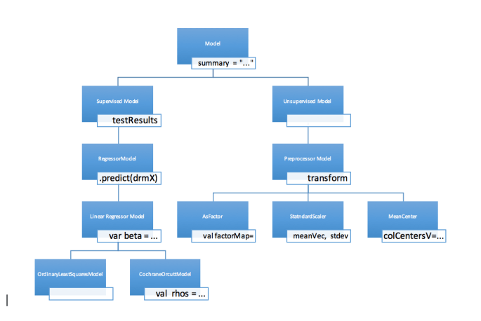
This isn’t a complete diagram but it is illustrative. For example- all Models have a summary string. All SupervisedModels have a Map of testResults. All RegressorModels have a .predict(...) method, and when ClassifierModel is introduced, they may have a .predict(...) method as well, or perhaps they will have a .classify(...) method.

Preprocessors are treated as unsupervised models. They must also be fit. Consider a StandardScaler, which must be “fit” on a data set to learn the mean and standard deviation.

The hierarchy of fitters is identical.

Hyper-parameter system

Hyper-parameters are passed in fitter functions as symbols. For example:

val model = new OrdinaryLeastSquares[Int]().fit(drmX, drmY, 'calcCommonStatistics → false)

Different methods have different hyper-parameters which maybe set. This method has advantages of extreme flexibility. It also side-steps the type safety of the Scala language, which depending on weather or not you like or hate type-safety, you might consider to be a good or bad thing. A notable draw back- if you pass a parameter that isn’t used by the method, it will be ignored silently, that is to say it will be ignored and it won’t warn you are throw an error. The real threat here is typos- where you think are doing something like, specifying an interceptless regression, however instead of specifying 'addIntercept -&gt; false you accidentally type 'addInterept -&gt; false, then the regression will add an intercept and throw no warnings that you’ve committed a typo. (This will possibly be fixed soon).

Also, in both hyperparameter examples given have had Boolean values, however the value can be anything. For example, in Cochrane-Orcutt on of the hyperparameters 'regressor can be any sub-class of LinearRegressorFitter!

In Practice

Preprocessors

There are currently three pre-processors available.
* AsFactor which is sometimes referred to as Dummy Variables or One-Hot encoder (Mahout chose R-semantics here over Python)
* StandardScaler which is goes by the same name in sklearn and the function scale in R.
* MeanCenter which is very similar to the standard scaler, however it only centers each column. In the future it is possible that MeanCenter will be combined with StandardScaler (as is done in R).

A preprocessor example

A fun tip: the unit tests of any package are full of great example. This one comes from: https://github.com/apache/mahout/blob/master/math-scala/src/test/scala/org/apache/mahout/math/algorithms/PreprocessorSuiteBase.scala

Setup Code
val A = drmParallelize(dense(
(3, 2, 1, 2),
(0, 0, 0, 0),
(1, 1, 1, 1)), numPartitions = 2)

// 0 -> 2, 3 -> 5, 6 -> 9
How to use AsFactor from Apache Mahout
val factorizer: AsFactorModel = new AsFactor().fit(A)
val factoredA = factorizer.transform(A)
val myAnswer = factoredA.collect
Check our results
println(factoredA)
println(factorizer.factorMap)
val correctAnswer = sparse(
svec((3 → 1.0) :: (6 → 1.0) :: (8 → 1.0) :: (11 → 1.0) :: Nil, cardinality = 12),
svec((0 → 1.0) :: (4 → 1.0) :: (7 → 1.0) :: ( 9 → 1.0) :: Nil, cardinality = 12),
svec((1 → 1.0) :: (5 → 1.0) :: (8 → 1.0) :: (10 → 1.0) :: Nil, cardinality = 12)
)
val epsilon = 1E-6
(myAnswer.norm - correctAnswer.norm) should be <= epsilon

The big call out from the above- is that the interface for this preprocessor (the second block of code) is exceptionally clean for a distributed, GPU accelerated, machine learning package.

Regressors

There are currently two regressors available:
* OrdinaryLeastSquares – Closed form linear regression
* Cochrane-Orcutt – A method for dealing with Serial Correlation

Oh, horay- another linear regressor for big data. First off- don’t be sassy. Second, OLS in Apache Mahout is closed form- that is to say, it doesn’t rely on Stochastic Gradient Descent to approximate the parameter space β.

Among other things, this means we are able to know the standard errors of our estimates and make a number of statistical inferences, such as the significance of various parameters.

For the initial release of the algorithms framework, OrdinaryLeastSquares was chosen because of its widespread familiarity. CochraneOrcutt was chosen for its relative obscurity (in the Big Data Space). The Cochrane Orcutt procedure is used frequently in econometrics to correct for auto correlation in the error terms. When auto-correlation (sometimes called serial-correlation) is present the standard errors are biased, and so is our statistical inference. The Cochrane Orcutt procedure attempts to correct for this.

It should be noted, implementations of Cochrane-Orcutt in many statistics packages such as R’s orcutt iterate this procedure to convergence. This is ill-advised on small data and big data alike. Kunter et. al recommend no more than three iterations of the Cochrane Orcutt procedure- if suitable parameters are not achieved, the user is advised to use another method to estimate ρ.

The point of implementing the CochraneOrcutt procedure was to show, that the framework is easily extendable to esoteric statistical/machine-learning methods, and users are encouraged to extend and contribute. Observe the implementation of the algorithm, and after groking, the reader will see that the code is quite expressive and tractable, and the majority of the fit method is dedicated to copying variables of interest into the resulting Model object.

A Regression Example
Setup Code
val alsmBlaisdellCo = drmParallelize( dense(
(20.96,  127.3),
(21.40,  130.0),
(21.96,  132.7),
(21.52,  129.4),
(22.39,  135.0),
(22.76,  137.1),
(23.48,  141.2),
(23.66,  142.8),
(24.10,  145.5),
(24.01,  145.3),
(24.54,  148.3),
(24.30,  146.4),
(25.00,  150.2),
(25.64,  153.1),
(26.36,  157.3),
(26.98,  160.7),
(27.52,  164.2),
(27.78,  165.6),
(28.24,  168.7),
(28.78,  171.7) ))

val drmY = alsmBlaisdellCo(::, 0 until 1)
val drmX = alsmBlaisdellCo(::, 1 until 2)
Cochrane-Orcutt
var coModel = new CochraneOrcutt[Int]().fit(drmX, drmY , ('iterations -> 2))
println(coModel.beta)
println(coModel.se)
println(coModel.rho)
Regression Tests

Unlike R and sklearn, all regression statistics should be considered optional, and very few are enabled by default. The rationale for this is that when working on big data, calculating common statistics could be costly enough that, unless the user explicitly wants this information, the calculation should be avoided.

The currently available regression tests are
* CoefficientOfDetermination – calculated by default, also known as the R-Square
* MeanSquareError – calculated by default, aka MSE
* DurbinWatson – not calculated by default, a test for the presence of serial correlation.

When a test is run, the convention is the following:

var model = ...
model = new MyTest(model)
model.testResults.get(myTest)

The model is then updated with the test result appended to the model’s summary string, and the value of the test result added to the model’s testResults Map.

Extending

Apache Mahout’s algorithm framework was designed to be extended. Even with the few example given, it should be evident that it is much more extensible than SparkML/MLLib and even sklearn (as all of the native optimization is abstracted away).

While the user may create their own algorithms with great ease- all are strongly encouraged to contribute back to the project. When creating a “contribution grade” implemenation of an algorithm a few considerations must be taken.

  1. The algorithm must be expressed purely in Samasara (The Mahout R-Like DSL). That is to say, the algorithm may not utilize any calls specific to an underlying engine such as Apache Spark.
  2. The algorithm must fit into the existing framework or extend the framework as necessary to ‘fit’. For example, we’d love to see a classification algorithm, but one would have to write the Classifier trait (similar to the Regressor trait).
  3. New algorithms must demonstrate a prototype in either R, sklearn, or someother package. That isn’t to say the algorithm must exist (though currently, all algorithms have an analgous R implementation). If there is no function that performs your algorithm, you must create a simple version in another language and include it in the comments of your unit test. This ensures that others can easily see and understand what it is that the algorithm is supposed to do.

Examples of number three are abound in the current unit tests. Example

Conclusions

Apache Mahout v0.13.0 offers a number of exciting new features, but the algorithms framework is (biasedly) one of my favorite. It is an entire framework that encourages statisticians and data scientists who have until now been intimidated by contributing to open source a green field opportunity to implement their favorite algorithms and commit them to a top-level Apache Software Foundation project.

There has been to date a mutually exclusive choice between ‘powerful, robust, and extendable modeling’ and ‘big data modeling’, each having advantages and disadvantages. It is my sincere hope and believe that the Apache Mahout project will represent the end of that mutual exclusivity.

Deep Magic, Volume 3: Eigenfaces

This week we’re going to really show off how easy it is to “roll our own” algorithms in Apache Mahout by looking at Eigenfaces. This algorithm is really easy and fun in Mahout because Mahout comes with a first class distributed stochastic singular value decomposition Mahout SSVD.

This is going to be a big job, and assumes you are have HDFS, and a small cluster to work with. You may be able to run this on your laptop, but I would recommend following the last post on setting up a small cloud-based hadoop cluster with Apache Zeppelin.

Eigenfaces are an image equivelent(ish) to eigenvectors if you recall your high school linear algebra classes. If you don’t recall: read wikipedia otherwise, it is a set of ‘faces’ that by a linear combination can be used to represent other faces.

Step 1. Get Data

The first thing we’re going to do is collect a set of 13,232 face images (250×250 pixels) from the Labeled Faces in the Wild data set.

Because some of these shell commands take a little while to run, it is worth taking a moment to set shell.command.timeout.millisecs in the sh interpreter to 600000.

My first paragraph, I’m going to make a directory for my final eigenface images that Zeppelin’s HTML loader can use. Then I’m going to download and untar the dataset. Finally, I’ll put the dataset into the tmp folder in HDFS.

%sh

mkdir zeppelin-0.7.0-SNAPSHOT/webapps/webapp/eigenfaces

wget http://vis-www.cs.umass.edu/lfw/lfw-deepfunneled.tgz
tar -xzf lfw-deepfunneled.tgz
hdfs dfs -put /home/guest/lfw-deepfunneled /tmp/lfw-deepfunneled

Step 2. Add dependency JARs

We use the Scala package scrimage to do our image processing, so we’ll want to add those jars. Also, there is a bug we’re working on in Mahout where broadcasting vectors doesn’t work so well in shell / Zeppelin mode. To get around this, I have added the transformer I need in custom jar of algorithms I use.

MAHOUT-1892: Broadcasting Vectors in Mahout-Shell

If that issue is still open, you’ll need to clone and build my branch (or make your own jar).

git clone https://github.com/rawkintrevo/mahout
cd mahout
git checkout mahout-1856
mvn clean package -DskipTests

Finally, assuming you are using Big Insights on Hadoop Cloud, you’ll need to copy the jar to the cluster.

scp algos/target/mahout-algos_2.10-0.12.3-SNAPSHOT.jar username@bi-hadoop-prod-XXX.bi.services.us-south.bluemix.net:/home/guest/mahout-algos_2.10-0.12.3-SNAPSHOT.jar

Changing username to your username and bi-hadoop-prod-XXX.bi.services.us-south.bluemix.net to your server address.

Back in Zeppelin, load the dependencies:

%sparkMahout.dep

z.load("com.sksamuel.scrimage:scrimage-core_2.10:2.1.0")
z.load("com.sksamuel.scrimage:scrimage-io-extra_2.10:2.1.0")
z.load("com.sksamuel.scrimage:scrimage-filters_2.10:2.1.0")

// add EXPERIMENTAL mahout algos
// https://github.com/rawkintrevo/mahout/tree/mahout-1856/algos
z.load("/home/guest/mahout-algos_2.10-0.12.3-SNAPSHOT.jar")

Step 3. Setup the Mahout Context

This step imports the Mahout packages and sets up the Mahout Distributed Context

%sparkMahout.spark

import org.apache.mahout.math._
import org.apache.mahout.math.scalabindings._
import org.apache.mahout.math.drm._
import org.apache.mahout.math.scalabindings.RLikeOps._
import org.apache.mahout.math.drm.RLikeDrmOps._
import org.apache.mahout.sparkbindings._

@transient implicit val sdc: org.apache.mahout.sparkbindings.SparkDistributedContext = sc2sdc(sc)

Step 4. Create a DRM of Vectorized Images

When doing image processing, we want a Matrix where each image is represented as a vector of numbers, where the number correspond to each pixel.

%sparkMahout.spark

import com.sksamuel.scrimage._
import com.sksamuel.scrimage.filter.GrayscaleFilter

val imagesRDD:DrmRdd[Int] = sc.binaryFiles("/tmp/lfw-deepfunneled/*/*", 500)
       .map(o => new DenseVector( Image.apply(o._2.toArray)
       .filter(GrayscaleFilter)
       .pixels
       .map(p => p.toInt.toDouble / 10000000)) )
   .zipWithIndex
   .map(o => (o._2.toInt, o._1))

val imagesDRM = drmWrap(rdd= imagesRDD).par(min = 500).checkpoint()

println(s"Dataset: ${imagesDRM.nrow} images, ${imagesDRM.ncol} pixels per image")

sc.binaryFiles is the spark way to read in our images. We set out partitioning to 500, and map each image into a scrimage object which drops the color information (we don’t need it for feature mapping) and converts the image to an array of large integers. We scale the integers down, and use the array to create a Mahout DenseVector. Finally we zipWithIndex and then use drmWrap to transform our RDD into a DRM.

Step 5. Subtract Means

IF vector broadcasting in the shell were working (it may be by the time you read this), this is how we would subtract our means.

%sparkMahout.spark

// How you would do this without help
// Doesn't work re BUG: MAHOUT-1892
val colMeansV = imagesDRM.colMeans
val bcastV = drmBroadcast(colMeansV)

val smImages = input.mapBlock(imagesDRM.ncol) {
case (keys, block) =>
      val copy: Matrix = block.cloned
      copy.foreach(row => row -= bcastV.value)
      (keys, copy)
}

We use the .colMeans method to get the colmeans, and then do a mapBlock on the images matrix, subtracting the mean from each image.

Since at the moment the above does not work, here is the hack to do it.

%sparkMahout.spark

// EXPERIMENTAL https://github.com/apache/mahout/pull/246
import org.apache.mahout.algos.transformer.SubtractMean

// Subtract Mean transforms each row by subtracting the column mean
val smTransformer = new SubtractMean()

smTransformer.fit(imagesDRM) // calculuates the column mean
val smImages = smTransformer.transform(imagesDRM) // return new DRM of subtracted means

smImages.checkpoint()

Again, this is only needed as a work around. If you’re interested in how easy it is to package your own functions into a jar- check out the SubtractMean source code

Step 6. Distributed Stochastic Singlar Value Decomposition

Based primarily on Nathan Halko’s dissertation most of the hard part here is done for us.

%sparkMahout.spark

import org.apache.mahout.math._
import decompositions._
import drm._

val(drmU, drmV, s) = dssvd(smImages, k= 20, p= 15, q = 0)

Here k is rank of the output e.g. the number of eigenfaces we want out. p is oversampling parameter, and q is the number of additional power iterations. Read Nathan’s paper or see ssvd docs for more information.

The above will take some time- about 35 minutes on a 5-node Big Insights Cloud Cluster.

drmV will be contain our Eigenfaces (transposed).

drmU will tell us the composition of each face we fed into the algorithm. For example

%sparkMahout

drmU.collect(0 until 1, ::)

yields

{0:-5.728272924185402E-4,1:0.005311020699576641,2:-0.009218182156949998,3:0.008125182744744356,4:0.001847134204087927,5:-0.01391318137456792,6:0.0038760898878500913,7:0.0022845256274037842,8:0.007046521884887152,9:0.004835772814429175,10:0.00338488781174816,11:0.009318311263249005,12:-0.005181665861179919,13:-0.004665157429436422,14:0.003072181956470255,15:-0.01285733757511248,16:0.005066140593688097,17:-0.016895601017982726,18:-0.012156252679821318,19:-0.008044144986630029 ... }

Which implies the first image = .005 * eigenFace1 + -.009 * eigenFace2 + …

Step 7. Write the Eigenfaces to disk

We want to SEE our eigenfaces! We use scrimage again to help us reconstruct our calculated eigenfaces back in to images.

%sparkMahout.spark

import java.io.File
import javax.imageio.ImageIO

val sampleImagePath = "/home/guest/lfw-deepfunneled/Aaron_Eckhart/Aaron_Eckhart_0001.jpg"
val sampleImage = ImageIO.read(new File(sampleImagePath))  
val w = sampleImage.getWidth
val h = sampleImage.getHeight

val eigenFaces = drmV.t.collect(::,::)
val colMeans = smImages.colMeans

for (i <- 0 until 20){
    val v = (eigenFaces(i, ::) + colMeans) * 10000000
    val output = new Array[com.sksamuel.scrimage.Pixel](v.size)
    for (i <- 0 until v.size) {
        output(i) = Pixel(v.get(i).toInt)
    }
    val image = Image(w, h, output)
    image.output(new File(s"/home/guest/zeppelin-0.7.0-SNAPSHOT/webapps/webapp/eigenfaces/${i}.png"))
}

First we load a sampleImage so we can get the height and width. I could have just opened it up in an Image viewer, but y’know, code. drmV has our eigenfaces as columns, so we transpose that. Also recall we subtracted the column means when we in-processed the images, so we’ll need to add that back.

We do a simple for loop over the eigenFaces, basically undoing the inprocessing we did. We then create an array of pixels, we do that by iterating through the vector. Finally we create the image with the width and height, and save it to the directory we set up. ZEPPELIN_HOME/webapps/webapp/ is the root directory for the %html interpreter, so we save our images in a directory there (we created this directory at the beginning).

Step 8. Display the Images

Scala is fun, but for simple string and list manipulation, I love Python

%python

r = 4
c = 5
print '%html\n<table style="width:100%">' + "".join(["<tr>" + "".join([ '<td><img src="eigenfaces/%i.png"></td>' % (i + j) for j in range(0, c) ]) + "</tr>" for i in range(0, r * c, r +1 ) ]) + '</table>'

All that does is create an html table of our images.

Screenshot from 2016-11-10 16-26-02.png

And that’s it!

I hope you enjoyed this one as much as I did, please leave comments and let me know how it went for you.

Big Data for n00bs: Gelly on Apache Flink

Big Data for n00bs is a new series I’m working on targeted at absolute beginners like my self.  The goal is to make some confusing tasks more approachable.  The first few posts will be spin offs of a recent talk I gave at Flink Forward 2016 Apache Zeppelin- A Friendlier Way To Flink (will link video when posted).

Graph databases are becoming an increasingly popular way to store and analyze data, especially when relationships can be expressed in terms of object verb objectFor instance, social networks are usually represented in graphs such as 

Jack likes Jills_picture

A full expose on the uses and value of graph databases is beyond the scope of this blog post however the reader is encouraged to follow these links for a more in depth discussion:


Gelly Library on Apache Flink

Gelly is the Flink Graph API.

Using d3js and Apache Zeppelin to Visualize Graphs

First, download Apache Zeppelin (click the link and choose the binary package with all interpreters) then “install” Zeppelin by unzipping the downloaded file and running bin/zeppelin-daemon.sh start or bin/zeppelin.cmd (depending on if you are using windows or Linux / OSX).  See installation instructions here.

After you’ve started Zeppelin, open a browser and go to http://localhost:8080

You should see a “Welcome to Zeppelin” page.  We’re going to create a new notebook by clicking the “Notebook” drop down, and the “+Create new note”.

screen-shot-2016-09-15-at-8-50-22-am

Call the notebook whatever you like.

Add dependencies to the Flink interpreter

Next we need to add two dependencies to our Flink interpreter.  To do this we go to the “Interpreters” page, find the “Flink” interpreter and add the following dependencies:

  • com.typesafe.play:play-json_2.10:2.4.8
    • used for reading JSONs
  • org.apache.flink:flink-gelly-scala_2.10:1.1.2
    • used for the Flink Gelly library

We’re also going to exclude com.typesafe:config from the typesafe dependency.  This packaged tends to cause problems and is not necessary for what we are doing, so we exclude it.

The dependencies section of our new interpreter will look something like this:

screen-shot-2016-09-15-at-8-58-08-am

Downloading some graph data

Go back to the notebook we’ve created.  In the first paragraph add the following code
%sh
mkdir tmp
wget https://raw.githubusercontent.com/d3/d3-plugins/master/graph/data/miserables.json -O tmp/miserables.json

It should look like this after you run the paragraph (clicking the little “play” button in top right corner of paragraph):

Screen Shot 2016-09-15 at 9.04.06 AM.png

What we’ve done there is use a Linux command wget to download our data. It is also an option to simply download the data your browser, you could for example right click on this link and click “Save As…” but if you do that, you’ll need to edit the next paragraph to load the data from where ever you saved it to.

Visualizing Data with d3js

d3js is a Javascript library for making some really cool visualizations. A fairly simple graph visualization was selected to keep this example fairly simple; a good next step would be to try a more advanced visualization.

First we need to parse our json:

import  scala.io.Source
import play.api.libs.json._
import org.apache.flink.graph.scala.Graph
import org.apache.flink.graph.Edge
import org.apache.flink.graph.Vertex

import collection.mutable._
import org.apache.flink.api.scala._

val dataJson = Source.fromFile("/home/guest/tmp/miserables.json").getLines.toList.mkString
val json: JsValue = Json.parse(dataJson)


Screen Shot 2016-09-20 at 12.10.02 PM.png
We’re going to have some output that looks like this/

For this hack, we’re going to render our d3js, by creating a string that contains our data.
(This is very hacky, but super effective).

%flinkGelly
println( s"""%html
<style>

.node {
  stroke: #000;
  stroke-width: 1.5px;
}

.link {
  fill: none;
  stroke: #bbb;
}

</style>
<div id="foo">


var width = 960,
    height = 300

var svg = d3.select("#foo").append("svg")
    .attr("width", width)
    .attr("height", height);

var force = d3.layout.force()
    .gravity(.05)
    .distance(100)
    .charge(-100)
    .size([width, height]);

var plot = function(json) {

  force
      .nodes(json.nodes)
      .links(json.links)
      .start();

  var link = svg.selectAll(".link")
      .data(json.links)
    .enter().append("line")
      .attr("class", "link")
    .style("stroke-width", function(d) { return Math.sqrt(d.value); });

  var node = svg.selectAll(".node")
      .data(json.nodes)
    .enter().append("g")
      .attr("class", "node")
      .call(force.drag);

  node.append("circle")
      .attr("r","5");

  node.append("text")
      .attr("dx", 12)
      .attr("dy", ".35em")
      .text(function(d) { return d.name });

  force.on("tick", function() {
    link.attr("x1", function(d) { return d.source.x; })
        .attr("y1", function(d) { return d.source.y; })
        .attr("x2", function(d) { return d.target.x; })
        .attr("y2", function(d) { return d.target.y; });

    node.attr("transform", function(d) { return "translate(" + d.x + "," + d.y + ")"; });
  });
}

plot( $dataJson )


</div>
""")

Now, check out what we just did there: println(s"""%html ... $dataJson. We just created a string that started with the %html tag, letting Zeppelin know, this is going to be a HTML paragraph, render it as such, and then passed the data directly in. If you were to inspect the page you would see the entire json is present in the html code.

Screen Shot 2016-09-20 at 12.20.35 PM.png
This is the (messy) graph we get.

From here, everything is a trivial exercise.

Let’s load this graph data into a Gelly Graph:

val vertexDS = benv.fromCollection(
(json \ "nodes" \\ "name")
.map(_.toString).toArray.zipWithIndex
.map(o => new Vertex(o._2.toLong, o._1)).toList)

val edgeDS = benv.fromCollection(
((json \ "links" \\ "source")
.map(_.toString.toLong) zip (json \ "links" \\ "target")
.map(_.toString.toLong) zip (json \ "links" \\ "value")
.map(_.toString.toDouble))
.map(o => new Edge(o._1._1, o._1._2, o._2)).toList)

val graph = Graph.fromDataSet(vertexDS, edgeDS, benv)

Woah, that looks spooky. But really is not bad. The original JSON contained a list called nodes which held all of our vertices, and a list called links which held all of our edges. We did a little hand waving to parse this into the format expected by Flink to create an edge and vertex DataSet respectively.

From here, we can do any number of graph operations on this data, and the user is encouraged to do more. For illustration, I will perform the most trivial of tasks: filtering on edges whose value is greater than 2.

val filteredGraph = graph.filterOnEdges(edge => edge.getValue > 2.0)

Now we convert our data back in to a json, and use the same method to re-display the graph. This is probably the most complex operation in the entire post.

val jsonOutStr = """{"nodes": [ """.concat(filteredGraph.getVertices.collect().map(v => """{ "name": """ + v.getValue() + """ } """).mkString(","))
.concat(""" ], "links": [ """)
.concat(filteredGraph.getEdges.collect().map(e => s"""{"source": """ + e.getSource() + """, "target": """ + e.getTarget + """, "value": """ + e.getValue + """}""").mkString(","))
.concat("] }")

As we see we are creating a json string from the edges and vertices of the graph. We call filteredGraph.getVertices.collect() and then map those vertices into the format expected by the json. In this case, our rendering graph expects a list of dictionaries of the format { "name" : }. The edges follow a similar pattern. In summation though we are simply mapping a list of of collected vertices/edges to string representations in a json format.

Finally, we repeat our above procedure for rendering this new json. An imporant thing to note, our code for mapping the graph to the json will work for this no matter what operations we perform on the graph. That is to say, we spend a little time setting things up, from a perspective of translating our graphs to jsons and rendering our jsons with d3js, and then we can play as much as we want with our graphs.

println( s"""
<style>

.node {
  stroke: #000;
  stroke-width: 1.5px;
}

.link {
  fill: none;
  stroke: #bbb;
}

</style>
<div id="foo2">


var width = 960,
    height = 500

var svg = d3.select("#foo2").append("svg")
    .attr("width", width)
    .attr("height", height);

var force = d3.layout.force()
    .gravity(.05)
    .distance(100)
    .charge(-100)
    .size([width, height]);

var plot = function(json) {

  force
      .nodes(json.nodes)
      .links(json.links)
      .start();

  var link = svg.selectAll(".link")
      .data(json.links)
    .enter().append("line")
      .attr("class", "link")
    .style("stroke-width", function(d) { return Math.sqrt(d.value); });

  var node = svg.selectAll(".node")
      .data(json.nodes)
    .enter().append("g")
      .attr("class", "node")
      .call(force.drag);

  node.append("circle")
      .attr("r","5");

  node.append("text")
      .attr("dx", 12)
      .attr("dy", ".35em")
      .text(function(d) { return d.name });

  force.on("tick", function() {
    link.attr("x1", function(d) { return d.source.x; })
        .attr("y1", function(d) { return d.source.y; })
        .attr("x2", function(d) { return d.target.x; })
        .attr("y2", function(d) { return d.target.y; });

    node.attr("transform", function(d) { return "translate(" + d.x + "," + d.y + ")"; });
  });
}

plot( $jsonOutStr )


</div>
""")

Also note we have changed $dataJson to $jsonOutStr as our new graph is contained in this new string.

A final important call out is the d3.select("#foo2") and <div id="foo2"> in the html string. This is creating a container for the element, and then telling d3js where to render the element. This was the hardest part for me; before I figured this out, the graphs kept rendering on the grey background behind the notebooks- which is cool, if that’s what you’re going for (custom Zeppelin skins anyone?), but very upsetting if it is not what you want.

Screen Shot 2016-09-20 at 12.31.44 PM.png
New filtered graph.

Conclusions

Apache Zeppelin is a rare combination of easy and powerful.  Simple things like getting started with Apache Flink and the Gelly graph library are fairly simple, however we are still able to add in powerful features such as d3js visualizations, with relatively little work.