
Big Data for n00bs is a new series I’m working on targeted at absolute beginners like my self. The goal is to make some confusing tasks more approachable. The first few posts will be spin offs of a recent talk I gave at Flink Forward 2016 Apache Zeppelin- A Friendlier Way To Flink (will link video when posted).
Graph databases are becoming an increasingly popular way to store and analyze data, especially when relationships can be expressed in terms of object verb object. For instance, social networks are usually represented in graphs such as
Jack likes Jills_picture
A full expose on the uses and value of graph databases is beyond the scope of this blog post however the reader is encouraged to follow these links for a more in depth discussion:
- Wikipedia- Graph Database
- IBM developerWorks- Processing large-scale graph data: A guide to current technology
- neo4j
Gelly Library on Apache Flink
Gelly is the Flink Graph API.
Using d3js and Apache Zeppelin to Visualize Graphs
First, download Apache Zeppelin (click the link and choose the binary package with all interpreters) then “install” Zeppelin by unzipping the downloaded file and running bin/zeppelin-daemon.sh start or bin/zeppelin.cmd (depending on if you are using windows or Linux / OSX). See installation instructions here.
After you’ve started Zeppelin, open a browser and go to http://localhost:8080
You should see a “Welcome to Zeppelin” page. We’re going to create a new notebook by clicking the “Notebook” drop down, and the “+Create new note”.
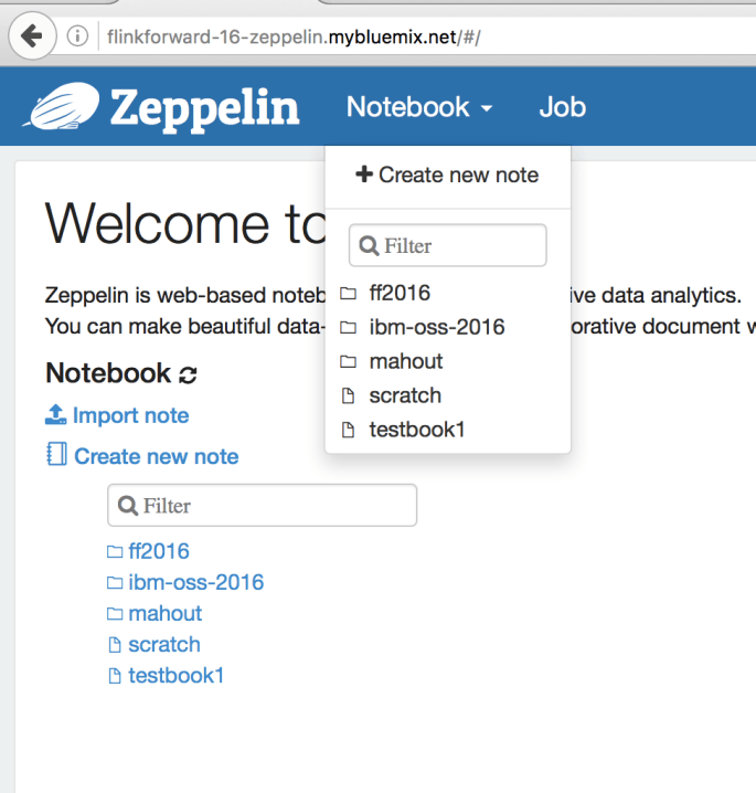
Call the notebook whatever you like.
Add dependencies to the Flink interpreter
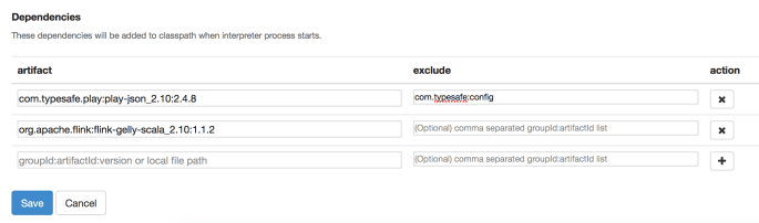
Next we need to add two dependencies to our Flink interpreter. To do this we go to the “Interpreters” page, find the “Flink” interpreter and add the following dependencies:
com.typesafe.play:play-json_2.10:2.4.8- used for reading JSONs
org.apache.flink:flink-gelly-scala_2.10:1.1.2- used for the Flink Gelly library
We’re also going to exclude com.typesafe:config from the typesafe dependency. This packaged tends to cause problems and is not necessary for what we are doing, so we exclude it.
The dependencies section of our new interpreter will look something like this:
Downloading some graph data
Go back to the notebook we’ve created. In the first paragraph add the following code
%sh

mkdir tmp

wget https://raw.githubusercontent.com/d3/d3-plugins/master/graph/data/miserables.json -O tmp/miserables.json
It should look like this after you run the paragraph (clicking the little “play” button in top right corner of paragraph):
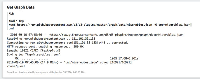
What we’ve done there is use a Linux command wget to download our data. It is also an option to simply download the data your browser, you could for example right click on this link and click “Save As…” but if you do that, you’ll need to edit the next paragraph to load the data from where ever you saved it to.
Visualizing Data with d3js
d3js is a Javascript library for making some really cool visualizations. A fairly simple graph visualization was selected to keep this example fairly simple; a good next step would be to try a more advanced visualization.
First we need to parse our json:
import  scala.io.Source
import play.api.libs.json._
import org.apache.flink.graph.scala.Graph
import org.apache.flink.graph.Edge
import org.apache.flink.graph.Vertex

import collection.mutable._
import org.apache.flink.api.scala._

val dataJson = Source.fromFile("/home/guest/tmp/miserables.json").getLines.toList.mkString
val json: JsValue = Json.parse(dataJson)
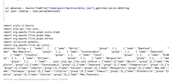
For this hack, we’re going to render our d3js, by creating a string that contains our data.
(This is very hacky, but super effective).
%flinkGelly
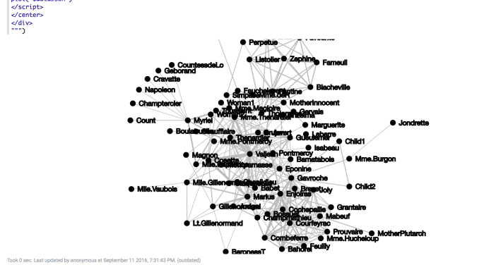
println( s"""%html
<style>
.node {
stroke: #000;
stroke-width: 1.5px;
}
.link {
fill: none;
stroke: #bbb;
}
</style>
<div id="foo">
var width = 960,
height = 300
var svg = d3.select("#foo").append("svg")
.attr("width", width)
.attr("height", height);
var force = d3.layout.force()
.gravity(.05)
.distance(100)
.charge(-100)
.size([width, height]);
var plot = function(json) {
force
.nodes(json.nodes)
.links(json.links)
.start();
var link = svg.selectAll(".link")
.data(json.links)
.enter().append("line")
.attr("class", "link")
.style("stroke-width", function(d) { return Math.sqrt(d.value); });
var node = svg.selectAll(".node")
.data(json.nodes)
.enter().append("g")
.attr("class", "node")
.call(force.drag);
node.append("circle")
.attr("r","5");
node.append("text")
.attr("dx", 12)
.attr("dy", ".35em")
.text(function(d) { return d.name });
force.on("tick", function() {
link.attr("x1", function(d) { return d.source.x; })
.attr("y1", function(d) { return d.source.y; })
.attr("x2", function(d) { return d.target.x; })
.attr("y2", function(d) { return d.target.y; });
node.attr("transform", function(d) { return "translate(" + d.x + "," + d.y + ")"; });
});
}
plot( $dataJson )
</div>
""")
Now, check out what we just did there: println(s"""%html ... $dataJson. We just created a string that started with the %html tag, letting Zeppelin know, this is going to be a HTML paragraph, render it as such, and then passed the data directly in. If you were to inspect the page you would see the entire json is present in the html code.
From here, everything is a trivial exercise.
Let’s load this graph data into a Gelly Graph:
val vertexDS = benv.fromCollection(
(json \ "nodes" \\ "name")
.map(_.toString).toArray.zipWithIndex
.map(o => new Vertex(o._2.toLong, o._1)).toList)

val edgeDS = benv.fromCollection(
((json \ "links" \\ "source")
.map(_.toString.toLong) zip (json \ "links" \\ "target")
.map(_.toString.toLong) zip (json \ "links" \\ "value")
.map(_.toString.toDouble))
.map(o => new Edge(o._1._1, o._1._2, o._2)).toList)

val graph = Graph.fromDataSet(vertexDS, edgeDS, benv)
Woah, that looks spooky. But really is not bad. The original JSON contained a list called nodes which held all of our vertices, and a list called links which held all of our edges. We did a little hand waving to parse this into the format expected by Flink to create an edge and vertex DataSet respectively.
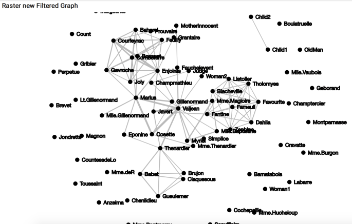
From here, we can do any number of graph operations on this data, and the user is encouraged to do more. For illustration, I will perform the most trivial of tasks: filtering on edges whose value is greater than 2.
val filteredGraph = graph.filterOnEdges(edge => edge.getValue > 2.0)
Now we convert our data back in to a json, and use the same method to re-display the graph. This is probably the most complex operation in the entire post.
val jsonOutStr = """{"nodes": [ """.concat(filteredGraph.getVertices.collect().map(v => """{ "name": """ + v.getValue() + """ } """).mkString(","))
.concat(""" ], "links": [ """)
.concat(filteredGraph.getEdges.collect().map(e => s"""{"source": """ + e.getSource() + """, "target": """ + e.getTarget + """, "value": """ + e.getValue + """}""").mkString(","))
.concat("] }")
As we see we are creating a json string from the edges and vertices of the graph. We call filteredGraph.getVertices.collect() and then map those vertices into the format expected by the json. In this case, our rendering graph expects a list of dictionaries of the format { "name" : }. The edges follow a similar pattern. In summation though we are simply mapping a list of of collected vertices/edges to string representations in a json format.
Finally, we repeat our above procedure for rendering this new json. An imporant thing to note, our code for mapping the graph to the json will work for this no matter what operations we perform on the graph. That is to say, we spend a little time setting things up, from a perspective of translating our graphs to jsons and rendering our jsons with d3js, and then we can play as much as we want with our graphs.
println( s"""
<style>

.node {
  stroke: #000;
  stroke-width: 1.5px;
}

.link {
  fill: none;
  stroke: #bbb;
}

</style>
<div id="foo2">


var width = 960,
    height = 500

var svg = d3.select("#foo2").append("svg")
    .attr("width", width)
    .attr("height", height);

var force = d3.layout.force()
    .gravity(.05)
    .distance(100)
    .charge(-100)
    .size([width, height]);

var plot = function(json) {

  force
      .nodes(json.nodes)
      .links(json.links)
      .start();

  var link = svg.selectAll(".link")
      .data(json.links)
    .enter().append("line")
      .attr("class", "link")
    .style("stroke-width", function(d) { return Math.sqrt(d.value); });

  var node = svg.selectAll(".node")
      .data(json.nodes)
    .enter().append("g")
      .attr("class", "node")
      .call(force.drag);

  node.append("circle")
      .attr("r","5");

  node.append("text")
      .attr("dx", 12)
      .attr("dy", ".35em")
      .text(function(d) { return d.name });

  force.on("tick", function() {
    link.attr("x1", function(d) { return d.source.x; })
        .attr("y1", function(d) { return d.source.y; })
        .attr("x2", function(d) { return d.target.x; })
        .attr("y2", function(d) { return d.target.y; });

    node.attr("transform", function(d) { return "translate(" + d.x + "," + d.y + ")"; });
  });
}

plot( $jsonOutStr )


</div>
""")
Also note we have changed $dataJson to $jsonOutStr as our new graph is contained in this new string.
A final important call out is the d3.select("#foo2") and <div id="foo2"> in the html string. This is creating a container for the element, and then telling d3js where to render the element. This was the hardest part for me; before I figured this out, the graphs kept rendering on the grey background behind the notebooks- which is cool, if that’s what you’re going for (custom Zeppelin skins anyone?), but very upsetting if it is not what you want.
Conclusions
Apache Zeppelin is a rare combination of easy and powerful. Simple things like getting started with Apache Flink and the Gelly graph library are fairly simple, however we are still able to add in powerful features such as d3js visualizations, with relatively little work.
